Assessing the Role of Oil Price Forecasts in Predicting Macroeconomic Indicators: A Conditional Forecasting Approach

Inam Ullah

doi:doi:10.11648/j.ijefm.20251303.16

Research Article |

| Peer-Reviewed

Assessing the Role of Oil Price Forecasts in Predicting Macroeconomic Indicators: A Conditional Forecasting Approach

Inam Ullah^*

Published in International Journal of Economics, Finance and Management Sciences (Volume 13, Issue 3)

Received: 22 April 2025 Accepted: 23 May 2025 Published: 30 June 2025

Views: Downloads:

Download PDF

Share This Article

Twitter
Linked In
Facebook

Abstract

This research endeavor carefully examines the economic effectiveness of oil price forecasts through the lens of conditional forecasting applied to three essential macroeconomic indicators—specifically, the Consumer Price Index (CPI), Industrial Production (IP), and Producer Price Index (PPI) within the United States. The analytical framework initially adopts a mixed sampling frequency approach to identify the trajectory of oil prices, utilizing high-frequency information to enhance the predictive process. Following this, macroeconomic conditional forecasts are methodically executed. Notably, the identified trends reflect a waning importance of oil price forecasts in relation to inflation predictions. Conversely, forecasts concerning price increases, manufacturing output, and the PPI reveal an inverse correlation. The complexities underlying this phenomenon are rigorously analyzed, with multiple plausible explanations presented. The robustness of our findings is highlighted by their consistency across various model specifications and forecasting methodologies, underscoring the reliability and durability of our analytical framework. Ultimately, this research offers critical insights into the intricate relationship between oil prices and macroeconomic variables, carrying significant implications for policymakers, businesses, and investors alike. The study elucidates the nuanced dynamics of oil price forecasts and their consequential effects on macroeconomic indicators, thereby not only enhancing the comprehension of economic interdependencies but also providing practical guidance for stakeholders navigating the intricate terrain of economic forecasting. The multifaceted implications of our findings extend beyond academic circles, positioning our research as a vital resource for those responsible for crafting informed policies, strategic business decisions, and investment strategies in the continuously evolving economic landscape.

Published in	International Journal of Economics, Finance and Management Sciences (Volume 13, Issue 3)
DOI	10.11648/j.ijefm.20251303.16
Page(s)	134-155
Creative Commons	This is an Open Access article, distributed under the terms of the Creative Commons Attribution 4.0 International License (http://creativecommons.org/licenses/by/4.0/), which permits unrestricted use, distribution and reproduction in any medium or format, provided the original work is properly cited.
Copyright	Copyright © The Author(s), 2025. Published by Science Publishing Group

Keywords

Macroeconomic Variables, Oil Price Volatility, High-frequency Data, Oil Price Forecasts

1. Introduction

This comprehensive study diligently tackles the essential endeavor of predicting the volatility of oil prices, which is an undertaking of utmost importance for any given economy given the profound and far-reaching effects such fluctuations have on inflation rates. The ability to foresee changes in volatility serves as a vital cornerstone for informed decision-making processes undertaken by policymakers, particularly in nations that are significantly dependent on oil revenues, such as the United States (U.S.). The precision and reliability of such forecasts take on an extraordinarily high level of importance for effective and strategic budgetary planning, which is crucial for maintaining economic stability. The dynamics of oil prices exert a considerable influence on a nation's international trade balances, thereby making the anticipation of these fluctuations an essential component for optimizing import-export strategies that countries may employ in a competitive global marketplace. Furthermore, businesses and investors utilize volatility forecasts as a means to effectively manage risks, formulate well-informed decisions, and adapt their strategies in response to the ever-changing conditions of the market landscape. Consumers, too, stand to gain significantly from these forecasts, as accurate predictions empower them to anticipate potential changes in energy costs, thus influencing their spending behaviors and financial planning in meaningful ways. Simultaneously, the overall stability of the global economy receives considerable bolstering through the practice of forecasting, enabling economies such as the U.S. to proactively prepare for possible economic spillovers and to mitigate the adverse effects that may arise from sudden and unexpected oil price fluctuations. Acknowledging the critical significance of oil price volatility forecasting, this study is meticulously designed to evaluate the predictive capabilities of oil prices, utilizing advanced econometric estimation methodologies that enhance the reliability of the findings. Importantly, this study emphasizes the economic value of these forecasts by employing conditional forecasting techniques that focus on key macroeconomic indicators, specifically the Consumer Price Index (CPI), Industrial Production (IP), and Producer Price Index (PPI) within the context of the U.S. economy, thereby contributing to a better understanding of the intricate relationships between oil prices and broader economic variables. Through these efforts, the study ultimately aims to provide a robust framework that informs various stakeholders about the implications of oil price volatility, enhancing their ability to respond effectively to economic challenges. In summary, the implications of this research extend well beyond mere academic interest, as they hold the potential to influence policy decisions, business strategies, and consumer behavior in a manner that fosters economic resilience and stability.

Extant research underscores the significance of forecasting oil prices for various stakeholders, including policymakers, enterprises, and households

[1]

. The pivotal role of oil prices in influencing multiple facets of economic activity and their consequential impact on the fiscal policies of oil-producing nations is well-documented. European financial markets, as highlighted by

[2]

, have been vigilant regarding the potential ramifications of low oil prices on achieving higher inflation rates. Similarly,

[3]

underscores concerns that continued declines in energy prices may precipitate a severe global economic downturn. Despite this acknowledged importance of oil price variations and projections, the existing literature has surprisingly overlooked the evaluation of the economic utility of these forecasts. Moreover, the study engages with the discourse on oil price volatility, emphasizing the necessity of employing model selection criteria, as opposed to relying solely on statistical testing, when determining the most suitable model specification for oil price analysis in the context of policymaking

[4]

. The assertion that accurate predictions of oil prices can enhance forecasts for various macroeconomic factors, thus potentially resulting in more effective policy measures, remains empirically unexamined. The study seeks to fill this gap by assessing and ranking modeling frameworks for oil prices based on their conditional performance in relation to a macroeconomic indicator.

Noteworthy is the current research focus on evaluating the effectiveness of oil price forecasting models, typically utilizing loss functions such as mean squared predictive error (MSPE) or mean absolute predictive error (MAPE) across various forecasting frameworks, including futures-based forecasts, fundamentals-based forecasts, and financial data-based forecasts

[5]

. The current study extends this paradigm by systematically assessing the relationship between the anticipated trajectory of petroleum prices and three critical macroeconomic indicators—CPI, IP, and PPI—utilized by policymakers to inform necessary adjustments for the U.S. economy. The study introduces a specific forecasting framework based on the correlation between

y_t

and

x_t

over time, wherein the exogenous variable x_t is related to the endogenous macroeconomic variable of interest,

y_t

. The primary aim is to demonstrate the significant role of oil prices in macroeconomic forecasting and furnish policymakers with a reliable framework for integrating oil prices into their projections. The unique framework enables more accurate predictions about the state of the U.S. economy, ultimately contributing to enhanced decision-making. The study, recognizing the multifaceted nature of macroeconomic indicators, commences by employing contemporary frameworks to predict oil prices, subsequently utilizing these predictions as assumptions for projecting the future trajectory of oil prices.

The contribution of this study is further underscored by the utilization of a Mixed Data Sampling (MIDAS) estimation architecture to anticipate the monthly prices of WTI crude oil. This approach incorporates predictive insights derived from WTI realized volatility measures and the WTI implied volatility index (OVX index). The motivation behind considering oil price volatility as a potential predictor of oil prices is anchored in the findings of

[6]

, highlighting the significant consequences of heightened volatility in oil prices for accurately forecasting future oil prices. This study, aligned with recent endeavors

[7]

, advocates for incorporating realized volatility derived from high-frequency data and oil price fundamentals at lower frequencies to enhance the accuracy of oil price forecasts.

The findings of this study unequivocally indicate that regardless of the forecasting methodology employed, projections of oil prices do not significantly enhance the accuracy of macroeconomic forecasts related to inflation. However, the study illuminates that the utilization of the MIDAS framework for oil price forecasting yields substantial enhancements in the accuracy of predictions for industrial production and the producer price index. The efficacy of variance risk premiums, particularly the disparity between realized and implied volatilities of oil prices, is demonstrated as a potential predictor for inflation expectations. The robustness tests confirm that macroeconomic predictions derived from MIDAS specifications outperform those generated by VAR and Bayesian VAR models in the context of oil price forecasts.

The subsequent sections of the article are meticulously organized, with Section 2 presenting a comprehensive Review of Literature. Section 3 provides a detailed exposition of Methods, Models, and Materials utilized in this study. Section 4 delves into the Results and Discussion, inclusive of a robustness analysis. Finally, Section 5 draws the study to a thoughtful conclusion, presenting several policy implications arising from the findings.

2. Literature Review

The repercussions of oil price shocks on diverse sectors of the economy have been extensively addressed within the expansive realm of research literature. Numerous studies have concentrated on oil-exporting nations, with the Organization of the Petroleum Exporting Countries (OPEC) assuming a central role in investigations seeking to quantify the ramifications of oil price shocks and volatility. The prevalent methodology for such analyses involves the utilization of vector autoregression (VAR) techniques, as evidenced by a majority of studies. In a similar vein,

[8]

delve into the causes of macroeconomic volatility in oil-producing nations, positing that oil price shocks exert a pronounced influence on the economic cycles of these countries. Examining the nexus between oil prices and government spending,

[9]

and

[10]

scrutinized 16 petroleum-exporting countries, discerning that oil prices play a pivotal role in shaping government budgetary priorities. Broadening the scope to encompass 40 oil-exporting nations,

[11]

explored the impact of oil price shocks on macroeconomic indicators, underlining the variability in effects contingent upon currency rate regimes and fiscal policy configurations.

The Gulf Cooperation Council (GCC) economies have not escaped scrutiny, with studies by

[12]

investigating the effects of oil price shocks on this regional bloc. Meanwhile,

[13]

discerned disparate impacts of petroleum price shocks on financial growth in the Middle East and North Africa.

[14]

focused on nations in the Caspian Basin, including Iran, Kazakhstan, and Russia, highlighting the substantial impact of sudden drops in oil prices on these countries. Similarly,

[15]

probed the repercussions of oil price fluctuations on Iran's macroeconomic indicators, identifying significant consequences such as currency depreciation, production losses, and inflationary pressures. In contrast,

[16]

posited that fluctuations in oil prices had minimal effects on the national economy of Nigeria. Shifting focus to Indonesia,

[17]

utilized an alternative methodology to conclude that oil prices could effectively forecast the trajectory of the Indonesian economy.

Global markets, too, have been under the analytical lens, with

[18]

scrutinizing the influence of petroleum costs on inflationary and manufacturing indices across the European Union. In China,

[19]

developed a computable general equilibrium (CGE) framework to assess the potential effects of global petroleum price fluctuations on Chinese businesses.

[20]

adopted a structure-based vector autoregression (VAR) framework, shedding light on the effects of crude pricing changes on the Chinese economic landscape.

[17]

utilized the vector error correction model (VECM) to explore the co-integrating connection between petroleum markets and global financial activity. In the realm of emerging methodologies, a burgeoning emphasis on machine learning technologies is evident.

[19]

introduced a decomposition-ensemble approach to enhance the precision of petroleum pricing projections, incorporating data-characteristic-driven restoration.

[20]

proposed the GA-NN technique, a fusion of evolutionary methods and neural networks, to forecast West Texas Intermediate (WTI) petroleum product prices and their relationship with economic indicators. This novel technique exhibited superior forecasting accuracy and computational efficiency compared to benchmark methods.

Markov paradigm-shifting frameworks were employed by

[21]

to investigate various modes of price behavior for Brent and WTI after the 2008 recession.

[22]

delved into the changing integration of the global petroleum market, utilizing a time-varying distance-average evaluation and a model for error correction. Gupta & Pierdzioch (2022) argued that price clustering could contribute to market inefficiencies, with their study focusing on five distinct types of oil futures contracts and uncovering indications of price clustering. Further innovation in artificial intelligence was introduced by

[23]

, who proposed a hybrid AI paradigm combining neural network algorithms and rule-driven systems for experts with online text extraction (WTM) approaches.

[24]

put forth the rough-set-refined data extraction (RSTM) technique, a data-driven forecasting approach designed to predict petroleum price patterns and their impact on economic indicators. Notably, these recent approaches underscore a paradigm shift towards utilizing advanced technologies in understanding the intricate relationship between oil prices and economic indicators.

In conclusion, the scientific exploration of oil price shocks spans diverse geographical and methodological dimensions, revealing nuanced impacts on national and global economies. This evolving landscape includes a transition towards leveraging cutting-edge technologies to enhance the precision of predictions and deepen our understanding of the complex interplay between oil prices and economic indicators.

3. Methods, Models, and Materials

The research methodology employed in this extensive examination engaged in a thorough and meticulous analysis of a wide array of data sourced from various reputable entities, most notably including the United States Energy Information Administration (EIA) and the Federal Reserve Economic Data (FRED) database, which are known for their reliability and comprehensive datasets. This carefully considered and discerning approach was specifically designed to extract not only nuanced insights but also solid empirical foundations that would serve as the bedrock for the subsequent investigation into the complex relationships at play. The intricate examination process incorporated the application of a variety of sophisticated statistical models, which encompassed regression analysis and time-series analysis, thereby enabling researchers to discern and quantify the multifaceted relationship between oil prices and critical macroeconomic indicators that have far-reaching implications. The study importantly recognizes that the volatility of oil prices acts as a pivotal linchpin in the forecasting efforts that are facilitated by these macroeconomic indicators, which are essential for informed decision-making. Acknowledging this significant aspect, the study positions itself at the forefront of contemporary research, striving to transcend established methodologies by integrating the complex dynamics of oil price fluctuations into existing forecasting models that are traditionally used. Through the strategic employment of advanced econometric estimation techniques, the study aspires not only to predict the future trajectory of economic indicators but also to significantly enhance the precision and reliability of these predictions, which is crucial for effective economic planning. The foresight into the volatility of oil prices, as facilitated by this innovative methodology, is expected to yield predictions that are more accurate, consequently fortifying the overall efficacy of macroeconomic forecasting models that rely on such data.

This methodological innovation is not merely an analytical pursuit undertaken in isolation; rather, it resonates with a broader purpose that seeks to underscore the profound significance of oil price variations within the larger context of macroeconomic forecasting endeavors. The intent behind this comprehensive study is crystal clear — to provide policymakers with a robust and trustworthy framework that transcends conventional paradigms, thereby enabling the seamless integration of oil prices into the intricate fabric of their economic projections and assessments. In the continually evolving landscape of economic dynamics, where the ability to foresee trends and changes is akin to currency, this methodological advancement stands poised to act as a catalyst for transformative decision-making processes that can lead to more effective governance. This methodological contribution serves as a testament to the unwavering commitment to excellence in research, where the relentless pursuit of knowledge converges harmoniously with the imperative of ensuring practical applicability in the real world. Furthermore, this study diligently follows the estimation procedures established by seminal research studies that have paved the way for further exploration in this critical area of economic inquiry, thereby solidifying its place in the ongoing discourse surrounding macroeconomic forecasting

[25]

3.1. Data and Materials

This study undertook an examination utilizing long-term monthly frequency data encompassing various critical variables. The chosen temporal scope for the monthly based analysis is deemed particularly suited for meticulous examination, thus aiding investors in their decision-making processes and portfolio management. The dataset spans from January 01, 1990, to August 30, 2020, providing a substantial timeframe for a comprehensive exploration. The study undertook a comprehensive examination of oil market volatility, leveraging both high and low-frequency data. For the creation of high-frequency measures of daily WTI volatility, we utilized data from front-month WTI futures contracts, which were transformed from ultra-high-frequency intraday time series. Our high-frequency forecasts relied on these volatility metrics, incorporating the daily prices of the OVX index (the implied volatility index for WTI) and the daily realized volatility measurements for WTI. The OVX implied volatility index data, essential for our study, was sourced from the CBOE, while tick-by-tick data was provided by Tick Data.

Furthermore, worldwide oil production and stockpiles statistics were acquired from the US Energy Information Administration, enhancing the depth of our analysis. Lutz Kilian's global economic activity index data, a key component of our research, was graciously supplied by the Federal Reserve Bank. The investigation focused on year-over-year variations in key economic indicators, namely the Consumer Price Index (CPI), the logarithm of industrial output, and the logarithm of the Producer Price Index (PPI), as visually represented in Figure 1. Figure 1 elucidates that the incorporation of oil price data into the analysis may result in diminished mean squared errors. Notably, the Root Mean Squared Error (RMSE) registers values below 1 for both Industrial Production (IP) and the Producer Price Index (PPI), with the latter exhibiting a more pronounced reduction. Conversely, examining the Consumer Price Index (CPI) reveals that the RMSE hovers around one at the commencement of the data time period. Subsequently, a noteworthy decline is observed until 2015, reaching a nadir of 0.86, indicative of a substantial influence of petroleum prices on the CPI during this period. While the pivotal role of oil prices in shaping the CPI is evident, a noteworthy observation is the upward trajectory in RMSE since 2015, suggesting a potential diminishing significance of oil prices in this context. This trend intimates that the economic utility of oil price estimates for predicting the CPI may be waning. The data paints a nuanced picture, suggesting that, despite the historical influence of oil prices on the CPI, their relevance may be diminishing in recent years. This outcome prompts a reconsideration of the economic efficacy of oil price estimates in the realm of CPI predictions, emphasizing the evolving nature of these interrelationships.

Download: Download full-size image

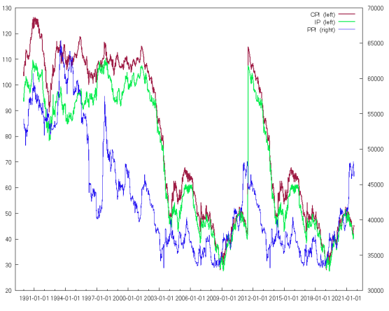
Figure 1. A pseudo-forecast oil price projection. Source: Author’s Calculation. Note: Comparison of the accuracy of oil-augmented prediction models to those without oil over 60 months.

3.2. Econometric Model Estimation

Let us assume that the exogenous variables,

x_{t}

, are related to the endogenous variable of interest,

y_{t}

, which is a macroeconomic variable. We establish a specific forecasting framework based on the correlation between

y_{t}

and

x_{t}

over time for US oil market.

y_{t} = f (x_{t - i}) + e_{t}

(1)

Here, to examining the above function in both cases (linear or non-linear) denoted as

f (x)

and an accompanying error term known as

e_{t}

, to gain insight into the macroeconomic variable that is dependent upon it. This requires a certain level of foresight and analytical prowess.

y_{t + h ∣ t} \equiv E (y_{t + h}| I_{t}),

(2)

The

I t

dataset accessible to the predictor at

time t

is vital in determining forecasts computed in the scenario where h is less than or equal to

i

y_{t + h ∣ t} = f (x_{t + h - i}) .

(3)

h

surpasses

i

, which is frequently the case, the predictions are unreliable.

y_{t + h ∣ t} = (f (x_{t + h - i ∣ t}) * d (h > i), f (x_{t + h - i}) * d (h \leq i))

(4)

When the inequality is valid, the function

d (f)

will have a value of 1, which indicates that

x_{t + h - i ∣ t}

is equivalent to

E (x_{t + h - i ∣ t}) .

Although the relationship between macroeconomic factors and oil prices may be either current

(i . e ., i = 0)

or have a time lag

(i . e ., i = 1 or 2)

, our focus is on computing projections of “macroeconomic variables from one month up to one year, at time t

+ h,

for

h \in [1, 12]

”. Hence, the currently accessible data set, t, is conditional. Therefore, predictions for “the dependent variable should only rely on the information available at time

t

to prevent forward-looking bias”. In this context, the term conditional forecasting is used. Similarly, the estimations for the relevant indicators are continued in the upcoming predictions which were presented in equations 5 to 19 respectively.

4. Results and Discussion

This study endeavors to quantify the predictive efficacy of oil prices on crucial macroeconomic indicators in the preceding decades. The focal point is a pseudo-forecast of three vital U.S. macroeconomic indicators—Consumer Price Index (CPI), Industrial Production (IP), and Producer Price Index (PPI)—all intricately linked to energy costs, particularly oil prices. This experimental foray involves forecasting IP and PPI based on crude oil price prognostications, utilizing a regression-based model and a Philips curve, respectively, to predict CPI. In this hypothetical scenario, this study affords the forecaster a forward-looking biased pseudo-forecast of oil prices. The analysis critically examines the capacity of current and past oil prices to effectively predict other macroeconomic indicators. Furthermore, nonlinear models are deployed to generate forecasts for these three macroeconomic variables. The evaluation metric employed is the ratio of the Root Mean Squared Error (RMSE) of the oil price projection to that of the other macroeconomic indicator for the ensuing month, serving as a yardstick for the "predictive" power of oil prices. A ratio below one signifies that models incorporating oil prices are deemed more accurate. This methodological approach delves into the intricate dynamics of oil prices and their influence on broader economic indicators, contributing valuable insights to the intersection of energy markets and macroeconomic forecasting.

4.1. Fuel Price Projection

To enhance the foresight of Consumer Price Index (CPI) projections, we employ the Philips curve in equation (14) considering both 3-variable and 12-lag "Bayesian VAR models." This investigation delves into the monthly impact on CPI projections, scrutinizing scenarios with and without oil price forecasts. The econometric models encompass a comprehensive consideration of oil market fundamentals, encompassing supply and demand dynamics, economic activity, and pricing mechanisms. The MSPE (Mean Squared Prediction Error) of CPI is meticulously presented in Table 1, differentiating between the enhanced Philips curve, which incorporates oil price estimates from the VAR and BVAR models, and the standard Philips curve devoid of these forecasts. This comparative analysis spans the actual out-of-sample forecasting period, offering a comprehensive view of forecasting accuracy. Moreover, the MCS (Model Confidence Set) test emerges as a pivotal tool in identifying the most effective models for CPI projection. This test assumes significance in affirming the efficacy of integrating oil price forecasts into inflation prediction models for enhanced accuracy. The outcomes underscore the instrumental role of the MCS test in discerning optimal models, emphasizing the imperative of incorporating oil price forecasts into the realm of inflation prediction methodologies.

Table 1. Conditional estimates of core CPI (MSPE for Forecasting Horizon).

$Model :$	$2 - months$	$4 - months$	$6 - months$	$8 - months$	$10 - months$
$Non – oil$	1.1205	1.2884	1.5117	2.7027	4.4215
$VAR (4, 13)$	1.1205	1.2882	1.5186	2.7489	4.4457
$BVAR (4, 13)$	1.1204	1.2882	1.5186	2.7189	4.4457

Note: The symbols “VAR (3,12) and BVAR (3,12)” signify that the models employ a 12-lag time series of information about oil yield, the global economic activity index, and the cost of oil.

This analysis unfolds through three dynamic econometric models: the non-oil model, VAR (4,13), and BVAR (4,13), spanning forecast horizons of two, four, six, eight, and ten months. The non-oil model reveals a notable increase in the mean squared prediction error (MSPE) with extended forecast horizons, signifying diminishing accuracy for core CPI predictions. While the MSPE is modest at two months (1.1205), it sharply rises to 4.4215 after ten months, emphasizing the superior accuracy of short-term forecasts. Similar trends are observed in the VAR (4,13) model, exhibiting an upward trajectory in MSPE values as the forecasting horizon lengthens. Discrepancies between the non-oil and VAR (4,13) models emerge, with the latter predicting a marginally higher MSPE (1.5186) at the six-month horizon. The inclusion of oil yield, global economic activity index, and oil prices enhances the VAR (4,13) model. The BVAR (4,13) model mirrors the MSPE trends of the VAR (4,13) model, with minor differences. For instance, both models exhibit an MSPE of 2.7189 and 2.7489 over an eight-month forecasting horizon. This suggests that the Bayesian approach does not significantly impact the accuracy of baseline CPI estimates, though it adds informational value.

The study concludes that, across all models, short-term core CPI estimates prove more reliable than long-term projections. While the inclusion of oil-related variables enhances certain aspects of the VAR models, it does not drastically improve prediction accuracy. Notably, the VAR and BVAR models cannot outperform the non-oil model in forecasting oil prices, indicating potential limitations in financial advantages when utilizing oil price predictions based on these models, particularly for the CPI. Figure 2 visually illustrates the efficiency of the BVAR model over time compared to the non-oil model, showcasing the Root Mean Squared Error (RMSE) between the basic and enhanced Philips curves. Additionally, Figure 2 represents Core Consumer Price Index projections using the BVAR model conditional on year-over-year shifts, providing insights into the model's forecasting ability over a 60-month moving average.

Download: Download full-size image

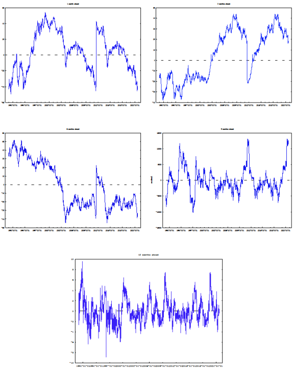
Figure 2. The core consumer price index (CPI) projections with utilizing monthly BVAR” conditional. Source: Author’s Calculation.

4.2. Macroeconomic Predictors

Consumer Price Index (CPI) is a measure that examines the average change in prices paid by consumers for a basket of goods and services over time. It is a key indicator of inflation and is widely used to assess changes in the cost of living for the average consumer. We employ monthly data spanning from January 2000 to August 2020, encompassing the US core Consumer Price Index (CPI) and the unemployment gap. The unemployment gap is derived by subtracting the actual unemployment rate from the rate it would be in the absence of inflation. In addition, the Industrial Production (IP) measures the output of industrial establishments, such as factories and mines. It quantifies the volume of production in the manufacturing, mining, and utilities sectors. IP is a crucial indicator of the overall health and performance of the industrial sector within an economy. Finally, the Producer Price Index (PPI) is an economic indicator that measures the average change over time in the selling prices received by domestic producers for their goods and services. It provides insight into the cost pressures at the producer level and is often considered a leading indicator of inflation, as changes in producer prices can influence consumer prices.

The data is sourced from the St. Louis Federal Reserve's authoritative Federal Reserve Economic Statistics. Additionally, monthly statistics on manufacturing output and the Producer Price Index (PPI) are included, enriching the dataset for a comprehensive analysis.

4.3. Inflation

Researchers frequently employ a revised Philips curve to evaluate how petroleum prices are influencing price increases. This technique aids in the evaluation of the correlation between the two variables.

φ (π_{t}) = a + \sum_{i = 1}^{I} β_{i} φ (π_{t - i}) + γ ({ungap}_{t - 1}) + \sum_{i = 0}^{I} δ_{i} φ ({Oil}_{t - i}) + e_{t}

(5)

The monthly core inflation rate,

π_{t}

, is influenced by several factors, including the unemployment gap in the United States,

{ungap}_{t}

, and the price of crude oil,

{Oil}_{t}

. The log levels, month-to-month and year-to-year shifts are all attributed to the function φ(.), which can take any form, whether linear or otherwise. The error term is represented by et∼N(0, σe2). Our approach is designed to encapsulate the current state of affairs and offer a thorough comprehension of the impact of rising oil prices on inflation during the Global Financial Crisis. Our objective is to contribute valuable insights to the existing knowledge on this subject, aiding policymakers in making well-informed decisions. Additionally, our methodology is characterized by novelty and innovation, and we anticipate its potential application in future research endeavors.

φ (π_{m, t + h}) = a + \sum_{i = 1}^{I} β_{i} φ (π_{t + h - i}) + γ ({ungap}_{t + h - 1}) + \sum_{i = 0}^{I} δ_{i} φ ({Oil}_{m, t + h - i ∣ t}) + e_{t + h}

(6)

Based on diverse oil price forecasting models, the genuine conditional projection of the core inflation is marked by the symbol πm, t+h. Here, m and h can be any integer between 1 and 12 months. The anticipated oil price for month

t + h

, based on each of the 14 models, is represented by

{Oil}_{m, t + h - i ∣ t}

. These models are based on six realized volatilities, the RVt (SJ), the OVX, and the six variance risk premiums. It must be noted that i ≥ h must be followed to prevent forward-looking bias. Using the data set accessible in month t, we can iteratively estimate oil price estimates for months’t + 1 through t + h. This approach can help forecast oil prices and make informed decisions about the oil industry.

{Oil}_{m, t + h ∣ t} = {Oil}_{m, t + h - 1 ∣ t} e^{(F_{t - i + h}^{'} β^{(t)} + \sum_{r = 0}^{k - 1} {VOL}_{(t - r - is)}^{' (D)} (\sum_{j = 0}^{p} r^{j} θ_{j}^{(t)}))},

(7)

at h≥2, whereas at h=1 we anticipate oil to be

{Oil}_{m, t + h ∣ t} = {Oil}_{t} e^{(F_{t - i + 1}^{'} β^{(t)} + \sum_{r = 0}^{k - 1} {VOL}_{(t - r - is)}^{' (D)} (\sum_{j = 0}^{p} r^{j} θ_{j}^{(t)}) + \frac{{\hat{σ}}_{ε}^{2}}{2})}

By inputting these numerical values into equation (6), we can ascertain which oil price estimate is more proficient in predicting the escalation of core inflation. To determine the most precise future oil price predictions, we employ the estimation of Eq. (6) for φ (πm, t), which comprises the logarithm of the consumer price index (CPIt), the monthly changes of CPIt, and the year-to-year changes of CPIt. We undertake this approach due to the uncertainty regarding which CPI series transformation will yield the most reliable outcomes.

4.4. Manufacturing Output and Supplier Price Indices

We compute the following formula to devise hypothetical predictions for industrial yield and the producer price index given petroleum price prognostications, akin to the method employed for inflation forecasts.

φ (z_{m, t + h}) = a + \sum_{i = 1}^{I} β_{i} φ (z_{t + h - i}) + \sum_{i = 0}^{I} δ_{i} φ ({Oil}_{m, t + h - i ∣ t}) + e_{t + h},

(8)

In the given equation, the precise conditional forecasts of oil prices in

“ month t + h ”

for either

IPt or PPIt

are represented by

zm and t + h

. The equation considers the forecast for oil prices in

month t + h

relied on the data from

month t

, denoted by

Oilm, t + h ∣ t

and the error term

et \sim N (0, σe 2)

. For robustness, we calculate the

m - o - m and y - o - y variations in IPt and PPIt

and the logarithmic levels, utilizing the estimated value of

φ (zm, t)

in Eq. (8).

By creating conditional estimates using non-oil models (equations (6) and (8), where oil price predictions are not taken into account), we can draw meaningful economic comparisons that are significant. This approach adds another layer of analysis to our findings, allowing for a more comprehensive understanding of the data at hand

\sum_{i = 0}^{I} δ_{i} φ ({Oil}_{m, t + h - i ∣ t})

4.5. Verification of Prediction Accuracy

Due to the highly nonlinear nature of the MIDAS model and following the recommendations of forecasting literature, we opted to employ the first half of the available data for the initial in-sample estimation period,

\overset{̆}{T}

(January 2010 - December 2014), and the second half for the out-of-sample evaluation period,

\overset{⃯}{T}

(January 2015 - December 2020)”. We utilize the Model Confidence Set (MCS) to select the most optimal models that exhibit an equivalent degree of prognosticating precision when predicting Indt: {πt, IPt, PPIt}, founded on evaluative standards for prediction. We utilize the most widely used statistical gauges of performance, the “Mean Squared Predictive Error (MSPE)” and the “Mean Absolute Predictive Error (MAPE).” To label the “

Ψ_{m, t}^{(mspe)}

and

Ψ_{m, t}^{(mape)}

” standards for assessment:

Ψ_{m, t}^{(mspe)} = {({Ind}_{m, t + h ∣ t} - {Ind}_{t + h})}^{2}

(9)

And

Ψ_{m, t}^{(mape)} = |{Ind}_{m, t + h ∣ t} - {Ind}_{t + h}|

(10)

Ind_{m, t+h∣t} represents a calculated approximation of the three significant economic indicators at

month t + h

, based on the accessible data at

month t

, considering the different oil price approximations from

model m

. The distinction between the errors in forecasting made by models m and m∗ can be identified for every month t,

d_{m, m^{*}, t} = Ψ_{m, t}^{(.)} - Ψ_{m^{*}, t}^{(.)}

the MCS test is conducted for every m, an element of M0 (the set comprising all competing methods). This test seeks to compare the hypothesis “

H 0, M : E (dm, m *, t) = 0, for V m, m * \in M, M \subset M 0

, against the alternative hypothesis

H 1, M : E (dm, m *, t) \neq 0, for some m, m * \in M .

” The performance of each model m is evaluated based on its mean out-of-sample rate of return (MSPE) and mean absolute percentage improvement (MAPE),

Ψ_{m}^{(.)} = {\overset{⃯}{T}}^{- 1} \sum_{t = 1}^{\overset{⃯}{T}} Ψ_{m, t}^{(.)}

4.6. Future Oil Price Predicting Using Realized Volatility (RV)

In the pursuit of refining financial modeling, we made predictions based on insights derived from existing literature, identifying seven realized volatility variations deemed to have the most significant impact. Each proposed metric brings its own set of advantages and disadvantages, with variations in the amount of information provided as explanatory variables. This meticulous approach aims to contribute valuable insights to the understanding of oil market dynamics and volatility, acknowledging the complexities inherent in financial modeling. The Realized Volatility (RVt) is defined as

[26]

{RV}_{t} = \sum_{i = 1}^{τ} r_{t, i}^{2}

(11)

The distinguished scholars

[27]

have made an outstanding contribution to the field of finance by introducing the concept of Realized Bi-power Variation

(RV t (b)) .

{RV}_{t}^{(b)} = {(2 / π)}^{- 1} (\frac{τ}{τ - 1}) \sum_{i = 1}^{τ - 1} |r_{t, i}| |r_{t, i + 1}|

(12)

Similarly, the median Realized Volatility (RV t(med)) describes a certain type of realized volatility.

{RV}_{t}^{(med)} = \frac{π}{6 - 4 \sqrt{3} + π} (\frac{τ}{τ - 2}) \sum_{i = 2}^{τ - 1} med {(|r_{t, i - 1}|, |r_{t, i}|, |r_{t, i + 1}|)}^{2}

(13)

The “Minimum Realized Volatility (RVt(min))” derived from the formula by

[28]

{RV}_{t}^{(\min)} = \frac{π}{π - 2} (\frac{τ}{τ - 1}) \sum_{i = 1}^{τ - 1} \min {(|r_{t, i}|, |r_{t, i + 1}|)}^{2} .

(14)

The

[29]

explores the concept of “Positive Semi Variance (RVt(+))” in a highly innovative and imaginative manner.

{RV}_{t}^{(+)} = \sum_{i = 1}^{τ} Ι \{r_{t, i} \geq 0\} r_{t, i}^{2},

(15)

If the input is precise and accurate, the function of the indicator I{.} will yield an output of 1, while in the event of an inaccuracy, it shall furnish a result of 0.

6. The concept of “Negative Semi Variance (RV t(-))”, as postulated by

[30]

, is a significant and intriguing one that warrants exploration and analysis.

{RV}_{t}^{(-)} = \sum_{i = 1}^{τ} Ι \{r_{t, i} < 0\} r_{t, i}^{2} .

(16)

All research on financial fluctuations that focus on predicting volatility relies on RV t, the initial approximation of intraday realized volatility based on a daily sampling frequency. This is the standard approach in all financial studies that forecasts market volatility.

When confronted with the presence of jumps, the estimation of integrated volatility IVt is carried out by

[31]

through “RV t(b).” Hence, the volatility comprises a jump component, and if the intraday asset price follows a jump-diffusion process, the quadratic variation “QVt” is equivalent to the integrated volatility added to the jump variation; or

{QV}_{t} = \int_{t - 1}^{t} σ_{s}^{2} ds + \sum_{t - 1 < s \leq t} κ_{s}^{2}

By amalgamating the realized variance and the power variation, impervious to the presence of jumps, assessing the constituents of the leap fluctuation is achievable.

Along with these realized volatility measures, we also consider the OVX index and variance risk premiums (VRP t)

[32]

, as well as the difference between the positive and negative semi-variance (RV t(sj) = RV t(+) RV t(-)).

{VRP}_{t} = {OVX}_{t} - {IRV}_{t}

(17)

OVXt represents the implied volatility of WTI. At the same time, IRVt pertains to any of the six available measures of intraday realized volatility - RVt, RVt(b), RVt(med), RVt(min), RVt(+), and RVt(-) - which are defined below.

4.7. Analysis of Oil Price Projections Based on CPI Forecast

We have devised a model to explain monthly changes in crude oil prices. Our model analyzes high-frequency data, specifically oil price volatility and low-frequency oil price fundamentals. We have employed a range of measures to capture the volatility of West Texas Intermediate (WTI) including RVt, RVt(b), RVt(med), RVt(min), RVt(+), RVt(−), RVt(sj), and the Oil Volatility Index (OVXt).

Table 2. Analysis of Petroleum Price Projections Based on Year-Over-Year Variations in Core CPI Projections.

$Model :$	$2 - months$	$4 - months$	$6 - months$	$8 - months$	$10 - months$
$Non - oil$	1.1098	1.1361	1.1732	1.1988	2.2259
$MIDAS - RV$	1.1101	1.139	1.182	2.2165	2.2421
$MIDAS - RV (b)$	1.1101	1.139	1.182	2.2165	2.2421
$MIDAS - RV (med)$	1.1101	1.139	1.182	2.2165	2.2421
$MIDAS - RV (\min)$	1.1101	1.139	1.182	2.2165	2.2421
$MIDAS - RV (-)$	1.1101	1.139	1.182	2.2165	2.2421
$MIDAS - RV (+)$	1.1101	1.139	1.182	2.2165	2.2421
$MIDAS - RV (sj)$	1.1101	1.139	1.182	2.2165	2.2421
$MIDAS - OVX$	1.1101	1.139	1.182	2.2165	2.2421
$MIDAS - VRP - RV$	1.1101	1.139	1.182	2.2165	2.2421
$MIDAS - VRP - RV (b)$	1.1101	1.139	1.182	2.2165	2.2421
$MIDAS - VRP - RV (med)$	1.1101	1.139	1.182	2.2165	2.2421
$MIDAS - VRP - RV (\min)$	1.1101	1.139	1.182	2.2165	2.2421
$MIDAS - VRP - RV (-)$	1.1101	1.139	1.182	2.2165	2.2421
$MIDAS - VRP - RV (+)$	1.1101	1.139	1.182	2.2165	2.2421

The representation of monthly returns on oil futures prices can be might be articulated as Δ(Oilt) = log(Oilt/Oilt−1)

F_{t} = {(\begin{matrix} {Gea}_{t}, & \log ({Prod}_{t} / {Prod}_{t - 1}), \end{matrix} \begin{matrix} \log ({Stocks}_{t} / {Stocks}_{t - 1}), & {Cap}_{t} \end{matrix})}^{'}

the fundamental recurring interval, occurring once each month, along with an array of elucidating elements represented as a vector

V O L_{(t)}^{(D)}

the “MIDAS model” is a sophisticated approach that involves RVt(sj), OVX, variance risk premiums, and the vector of realized volatilities. The model is designed to enable the monthly dependent variable to be correlated with the monthly explanatory variables, Ft, as well as the daily realized volatilities, VOL(t)(D), by utilizing the polynomial distributed lag weighting technique.

Δ ({Oil}_{t}) = F'_{t - i} β + \sum_{r = 0}^{k - 1} {VOL}_{(t - r - is)}^{' (D)} (\sum_{j = 0}^{p} r^{j} θ_{j}) + ε_{t}

(18)

Assuming a standard distribution for the error component, we designate εt∼N(0, σε2), with β, θj, and the assumed s = 22 signifying the count of daily observations for each month. Two pivotal factors influence current-month oil futures prices—past oil price fundamentals and preceding trading day volatility measures. Through meticulous variable construction and establishment of their relationship with the dependent variable, we eliminate potential bias, enabling prediction of oil futures prices up to a month in advance. Utilizing i = 1 (and is = 22) for predicting next month's oil price and i = 6 for forecasting six months into the future.

Table 2 showcase the conditional CPI projections. Initial observations reveal that various MIDAS models yield similar predictions, with no single specification standing out. Notably, the non-oil model consistently ranks among the best models across all prediction horizons, as evidenced by the MCS test. In Table 2, we scrutinize petroleum price forecasts concerning anticipated changes in the core Consumer Price Index (CPI) during the forecasting horizon. The table contrasts MSPE (Mean Squared Prediction Error) values among various models over different prediction horizons.

As the forecast time horizon extends, MSPE values for petroleum price estimates grow, suggesting decreasing reliability over time. The "non-oil" model consistently produces the lowest MSPE values, indicating superior performance in forecasting petroleum prices compared to other models. In contrast, the "MIDAS - RV" model and its subdivisions exhibit consistent MSPE values, implying limited enhancement in accuracy over the base "MIDAS - RV" model. Contrary to claims by So et al. (2022) regarding short-term oil price fluctuations' impact on price stability, our results do not support this view. Instead, findings align with research by Zheng et al. (2022), suggesting a diminishing influence of oil prices on inflation over time. Information from Table 2 implies that basing CPI projections on petroleum price predictions may lack financial benefit, possibly attributed to the diminished significance of oil prices in recent years due to more energy-efficient consumption patterns and improved monetary tools in the United States, as proposed by So et al. (2022).

4.8. Analysis of conditional IP Projections

Examining IPD projections under varied assumptions, Table 3 displays findings contributing to the ongoing discourse on oil price impacts on inflation rates. This study introduces fresh insights while corroborating prior research. Table 3 illustrates conditional Industrial Production (IP) estimates based on year-to-year oil price changes. Mean Squared Prediction Error (MSPE) serves for assessment across 2 to 10 months of predicting horizons. Statistics reveal the MIDAS - RV model surpasses the non-oil model across all horizons, offering higher accuracy and precision. Variants of MIDAS - RV yield comparable results, implying consistency in predicting IP based on oil price changes.

Table 3. Conditional IP projection evaluations using year-over-year variations in oil prices.

$Model :$	$2 - months$	$4 - months$	$6 - months$	$8 - months$	$10 - months$
$Non - oil$	1.5265	2.8088	6.6543	4.4466	31.9055
$MIDAS - RV$	1.418	2.8471	2.2332	4.4437	11.6204
$MIDAS - RV (b)$	1.4179	2.8471	2.2025	2.6432	12.92
$MIDAS - RV (med)$	1.4179	2.8471	2.2024	2.8419	12.9201
$MIDAS - RV (\min)$	1.4179	2.8471	2.2024	2.5426	12.92
$MIDAS - RV (-)$	1.4179	2.8471	2.2029	2.8433	13.3196
$MIDAS - RV (+)$	1.418	2.8471	2.2028	2.8443	14.4177
$MIDAS - RV (sj)$	1.418	2.8472	2.2025	2.8438	12.2136
$MIDAS - OVX$	1.4179	2.8471	2.2028	2.6415	12.2173
$MIDAS - VRP - RV$	1.4179	0.9474	2.2036	2.6431	13.3176
$MIDAS - VRP - RV (b)$	1.4179	2.847	2.2031	2.8422	13.3161
$MIDAS - VRP - RV (med)$	1.4179	2.8471	2.203	2.8418	13.3175
$MIDAS - VRP - RV (\min)$	1.4179	2.8471	2.203	2.9424	13.3162
$MIDAS - VRP - RV (-)$	1.4178	2.847	2.2035	2.5423	13.3133
$MIDAS - VRP - RV (+)$	1.4179	2.8469	2.203	2.5433	13.316

"MIDAS - VRP - RV" models exhibit varying success with the inclusion of VIX Futures Curve Risk Premium (VRP). At the 4-month horizon, this model outperforms MIDAS - RV and Non-oil models. However, contradictory findings emerge across horizons, with some variants excelling and others lagging compared to MIDAS - RV.

In conclusion, the MIDAS - RV model excels in predicting IP changes in response to oil price shifts, particularly for short- to medium-term forecasts. Some "MIDAS - VRP - RV" variants display notable accuracy gains with VRP, requiring further research. Contrary to Table 2, oil price forecasts show more significant predictive enhancements than the non-oil model. The "MCS test" indicates the non-oil model does not consistently rank among the best. No single "MIDAS model" stands out, suggesting high-frequency oil price volatility data's economic utility for IP forecasts, regardless of form or metric. Benefits range from 18% to 80% depending on the forecasting horizon, confirming Gong et al. (2022) assertion of oil price volatility's substantial impact on manufacturing output post-mid-1970s.

4.9. Analysis of Conditional PPI and Core CPI Projections

Table 4 presents the outcomes derived from employing the Producer Price Index (PPI) as our ultimate macroeconomic indicator. Our approach, as evidenced by the empirical results, demonstrates practicality and reliability, offering a means to accurately forecast future oil prices with significant economic implications. The results shown in Table 4 indicate that our "MIDAS-based" oil price projections exhibit the potential to enhance PPI predictions, showcasing promise in this domain. However, akin to the Industrial Production (IP), we refrain from designating a singular "best-in-class" "MIDAS model." Despite this, it is noteworthy that oil price predictions yield substantial forecasting improvements, with select models exhibiting up to a 94% enhancement compared to non-oil models. Our findings further reveal that "oil price projections offer more economic benefits for IP and PPI than for CPI," aligning with the initial results outlined in Section 3. We posit that oil prices exert a pronounced impact on production costs, the PPI index, and overall industrial output.

Table 4. Conditional PPI projections based on fluctuations from one year to the next.

$Model :$	$2 - months$	$4 - months$	$6 - months$	$8 - months$	$10 - months$
$Non - oil$	2.2697	14.4131	41.1072	71.163	111.1028
$MIDAS - RV$	3.3038	2.2781	1.1366	5.5226	5.5373
$MIDAS - RV (b)$	2.2037	2.2792	4.4401	5.5288	5.5396
$MIDAS - RV (med)$	2.204	2.279	4.3391	5.5281	5.5375
$MIDAS - RV (\min)$	2.2038	2.2792	4.3393	5.529	5.5385
$MIDAS - RV (-)$	2.2038	2.2785	4.3353	5.5314	5.5399
$MIDAS - RV (+)$	2.204	2.2778	4.3351	5.5291	5.5317
$MIDAS - RV (sj)$	2.2036	2.2765	4.3386	5.5411	5.5191
$MIDAS - OVX$	2.2038	2.2773	4.3377	5.5282	5.5316
$MIDAS - VRP - RV$	2.2039	2.2773	4.3404	5.5347	5.5435
$MIDAS - VRP - RV (b)$	2.2039	2.2787	4.3461	5.5374	5.5601
$MIDAS - VRP - RV (med)$	2.2042	2.2794	4.3439	5.5369	5.5598
$MIDAS - VRP - RV (\min)$	2.2042	2.2796	4.3446	5.5392	5.5596
$MIDAS - VRP - RV (-)$	2.2039	2.2783	4.3391	5.5384	5.5439
$MIDAS - VRP - RV (+)$	2.2037	2.2767	4.3364	5.5345	5.534

Table 5 delves into core Consumer Price Index (CPI) conditional estimations vis-à-vis diverse oil price forecasts, presenting Mean Squared Prediction Error (MSPE) across three distinct periods (in months) and corresponding to various MSPE measures: log-level data, month-over-month, and year-over-year changes. A holistic examination of the results unveils variability contingent on the model and time horizon. For instance, at a 2-month forecasting horizon, the "non-oil" model registers an MSPE of 1.1252, and the "MIDAS - RV" model records an MSPE of 1.1317 for log-level data forecasts. MSPE values fluctuate as the forecasting horizon extends, illustrating the models' diverse accuracy trajectories over time. While certain models outperform others across various periods and data transformations, it is imperative to consider the unique context and objectives of the analysis before drawing definitive conclusions.

4.10. Analysis of IP and PPI Conditional Forecasts

Table 6 presents the outcomes of examining projected petroleum prices based on Industrial Production (IP) conditional projections. Mean Squared Prediction Error (MSPE) is utilized to assess model precision across varying month-long prediction horizons. The "non-oil" model outperforms the "MIDAS - RV" model on all time horizons for log-level data, with the "Non-oil" model proving more reliable as forecasting horizons extend. The "MIDAS - RV (med)" model exhibits the lowest month-over-month (m-o-m) MSPE at the 1-month and 3-month forecasting timeframes, while the "non-oil" model excels for 6 months and beyond. For year-over-year changes, the "MIDAS - RV(b)" model shows the smallest MSPE for 1, 3, and 6-month forecasting horizons, while the "non-oil" model is most accurate at 9 and 12 months into the future. The shift in the weight of services in the US Consumer Price Index (CPI) calculation could explain why oil price projections offer predictive information for the Producer Price Index (PPI) but not the CPI. This is attributed to the decreasing prominence of manufacturing items, many of which use oil, in the CPI, while the weight of services has increased.

Table 5. Conditional Estimates of Core CPI To Evaluate Oil Price Projections.

MSPE – (Log)					MSPE – (Monthly Effect)				(MSPE –Yearly Effect)
Model:	2	4	7	10	2	4	7	10	2	4	7	10
𝑁𝑜𝑛 − 𝑜𝑖𝑙	1.1252	1.2071	1.2813	1.1829	1.2253	1.2764	1.1461	2.2631	1.1361	1.1732	1.1988	2.2259
𝑀𝐼𝐷𝐴𝑆 − 𝑅𝑉	1.1317	1.2659	1.2238	1.1906	1.2135	1.2584	1.1345	2.2692	1.139	1.182	1.2165	2.2421
𝑀𝐼𝐷𝐴𝑆 − 𝑅𝑉(𝑏)	1.1317	1.2659	1.2236	1.1905	1.2135	1.2584	1.1345	2.2692	1.139	1.182	1.265	2.2421
𝑀𝐼𝐷𝐴𝑆 − 𝑅𝑉(𝑚𝑒𝑑)	1.1317	1.2659	1.2236	1.1903	1.2135	1.2584	1.1345	2.2692	1.139	1.182	1.265	2.2421
𝑀𝐼𝐷𝐴𝑆 − 𝑅𝑉(𝑚𝑖𝑛)	1.1317	1.2659	1.2236	1.1905	1.2135	1.2584	1.1345	2.2692	1.139	1.182	1.265	2.2421
𝑀𝐼𝐷𝐴𝑆 − 𝑅𝑉(−)	1.1317	1.2659	1.2236	1.1906	1.2135	1.2584	1.1346	2.2692	1.139	1.182	1.265	2.2421
𝑀𝐼𝐷𝐴𝑆 − 𝑅𝑉(+)	1.1317	1.2659	1.2236	1.1907	1.2135	1.2584	1.1345	2.2692	1.139	1.182	1.265	2.2421
𝑀𝐼𝐷𝐴𝑆 − 𝑅𝑉(𝑠𝑗)	1.1317	1.2659	1.2236	1.1909	1.2135	1.2584	1.1345	2.2692	1.139	1.182	1.265	2.2421
𝑀𝐼𝐷𝐴𝑆 − 𝑂𝑉𝑋	1.1317	1.2659	1.2236	1.1909	1.2135	1.2584	1.1345	2.2692	1.139	1.182	1.265	2.2421
𝑀𝐼𝐷𝐴𝑆 − 𝑉𝑅𝑃 − 𝑅𝑉	1.1317	1.2659	1.2239	1.1909	1.2135	1.2584	1.1345	2.2692	1.139	1.182	1.265	2.2421
𝑀𝐼𝐷𝐴𝑆 − 𝑉𝑅𝑃 − 𝑅𝑉(𝑏)	1.1317	1.2659	1.2238	1.1909	1.2135	1.2584	1.1345	2.2692	1.139	1.182	1.265	2.2421
𝑀𝐼𝐷𝐴𝑆 − 𝑉𝑅𝑃 − 𝑅𝑉(𝑚𝑒𝑑)	1.1317	1.2659	1.2238	1.1909	1.2135	1.2584	1.1345	2.2692	1.139	1.182	1.265	2.2421
𝑀𝐼𝐷𝐴𝑆 − 𝑉𝑅𝑃 − 𝑅𝑉(𝑚𝑖𝑛)	1.1317	1.2659	1.2238	1.1909	1.2135	1.2584	1.1345	2.2692	1.139	1.182	1.265	2.2421
𝑀𝐼𝐷𝐴𝑆 − 𝑉𝑅𝑃 − 𝑅𝑉(−)	1.1317	1.2659	1.2238	1.1909	1.2135	1.2584	1.1345	2.2692	1.139	1.182	1.265	2.2421
𝑀𝐼𝐷𝐴𝑆 − 𝑉𝑅𝑃 − 𝑅𝑉(+)	1.1317	1.2659	1.2238	1.1909	1.2135	1.2584	1.1345	2.2692	---	---	---	---

Table 6. Analysis Of Petroleum Price Estimates Using IP Conditional Forecasts.

MSPE – (Log)					MSPE – (Monthly Effect)				(MSPE –Yearly Effect)
Model:	2	4	7	10	2	4	7	10	2	4	7	10
𝑁𝑜𝑛 − 𝑜𝑖𝑙	1.1111	3.3025	1.1031	4.4453	1.2398	2.2185	1.1679	4.4179	1.2265	2.8088	4.4543	7.7466
𝑀𝐼𝐷𝐴𝑆 − 𝑅𝑉	1.1069	2.239	1.1478	4.4049	1.2403	2.2388	1.1053	4.4583	1.118	2.8471	2.2032	2.8437
𝑀𝐼𝐷𝐴𝑆 − 𝑅𝑉(𝑏)	1.1069	2.239	1.1477	4.4045	1.2403	2.2388	1.1051	4.4583	1.1179	2.8471	2.2025	2.8432
𝑀𝐼𝐷𝐴𝑆 − 𝑅𝑉(𝑚𝑒𝑑)	1.1069	2.239	1.1477	4.4045	1.2403	2.2388	1.1051	4.4582	1.1179	2.8471	2.2024	2.8419
𝑀𝐼𝐷𝐴𝑆 − 𝑅𝑉(𝑚𝑖𝑛)	1.1069	2.239	1.1477	4.4043	1.2403	2.2388	1.1051	4.4583	1.1179	2.8471	2.2024	2.8426
𝑀𝐼𝐷𝐴𝑆 − 𝑅𝑉(−)	1.1069	2.239	1.1477	4.4044	1.2403	2.2388	1.1051	4.4581	1.1179	2.8471	2.2029	2.8433
𝑀𝐼𝐷𝐴𝑆 − 𝑅𝑉(+)	1.1069	2.239	1.1477	4.4047	1.2403	2.2388	1.1051	4.4584	1.118	2.8471	2.2028	2.843
𝑀𝐼𝐷𝐴𝑆 − 𝑅𝑉(𝑠𝑗)	1.1069	2.239	1.1477	4.4036	1.2403	2.2388	1.1051	4.4584	1.118	2.8471	2.2025	2.843
𝑀𝐼𝐷𝐴𝑆 − 𝑂𝑉𝑋	1.1069	2.239	1.1477	4.4046	1.2403	2.2387	1.1051	4.4584	1.1179	2.8471	2.2028	2.843
𝑀𝐼𝐷𝐴𝑆 − 𝑉𝑅𝑃 − 𝑅𝑉	1.1069	2.239	1.1478	4.4043	1.2403	2.2388	1.1054	4.4584	1.1179	2.8471	2.2036	2.843
𝑀𝐼𝐷𝐴𝑆 − 𝑉𝑅𝑃 − 𝑅𝑉(𝑏)	1.1069	2.239	1.1475	4.4043	1.2403	2.2387	1.1053	4.4584	1.1179	2.8471	2.2031	2.843
𝑀𝐼𝐷𝐴𝑆 − 𝑉𝑅𝑃 − 𝑅𝑉(𝑚𝑒𝑑)	1.1069	2.239	1.1475	4.4043	1.2403	3.3388	1.1052	4.4584	1.1179	2.8471	2.203	2.843
𝑀𝐼𝐷𝐴𝑆 − 𝑉𝑅𝑃 − 𝑅𝑉(𝑚𝑖𝑛)	1.1069	2.239	1.1475	4.4037	1.2403	2.2388	1.1052	4.4584	1.1179	2.8471	2.203	2.8424
𝑀𝐼𝐷𝐴𝑆 − 𝑉𝑅𝑃 − 𝑅𝑉(−)	1.1069	2.239	1.1475	4.404	1.2403	2.2387	1.1052	4.4584	1.1179	2.847	2.2035	2.8423
𝑀𝐼𝐷𝐴𝑆 − 𝑉𝑅𝑃 − 𝑅𝑉(+)	1.1069	2.239	1.1475	4.4044	1.2403	2.2387	1.1052	7.4	---	---	---	---

These findings underscore that projecting oil prices against core inflation expectations does not yield predictive advantages. While optimistic about the potential of "MIDAS-based" oil price projections in enhancing PPI predictions, refinement work on these models is essential. As forecasting horizons increase, MSPE values rise across all models, indicating a decline in accuracy over extended periods. The "MSPE - m-o-m changes" column highlights varying MSPE values from one month to the next, emphasizing diverse predictive accuracies among models. Similarly, Table 7 where the "MSPE - y-o-y changes" column depicts an overall increase in MSPE values with longer prediction horizons, indicating greater challenges in predicting annual gasoline price fluctuations over extended periods. Models like MIDAS RV(b), MIDAS RV (med), and MIDAS RV (min) consistently exhibit superior predictive ability with lower MSPE values across all three columns.

Table 7. Analysis Of Petroleum Price Projections Using PPI Conditional Projections.

MSPE – (Log)					MSPE – (Monthly Effect)				(MSPE –Yearly Effect)
Model:	2	4	7	10	2	4	7	10	2	4	7	10
𝑁𝑜𝑛 − 𝑜𝑖𝑙	1.159	13.346	21.115	36.662	2.316	8.86	25.565	34.553	2.27	15.513	42.207	72.263
𝑀𝐼𝐷𝐴𝑆 − 𝑅𝑉	1.179	13.349	41.108	65.555	2.39	3.409	13.378	14.488	2.604	4.478	4.237	5.523
𝑀𝐼𝐷𝐴𝑆 − 𝑅𝑉(𝑏)	1.179	13.349	41.166	63.337	2.39	3.408	13.378	14.486	2.604	4.179	4.237	5.529
𝑀𝐼𝐷𝐴𝑆 − 𝑅𝑉(𝑚𝑒𝑑)	1.179	13.348	41.167	64.411	2.39	3.408	13.377	14.486	2.604	4.179	4.237	5.528
𝑀𝐼𝐷𝐴𝑆 − 𝑅𝑉(𝑚𝑖𝑛)	1.18	13.348	41.166	64.427	2.39	3.408	13.378	14.486	2.604	4.179	4.237	5.529
𝑀𝐼𝐷𝐴𝑆 − 𝑅𝑉(−)	1.179	13.349	41.176	64.447	2.39	3.409	13.379	14.487	2.604	4.178	4.237	5.531
𝑀𝐼𝐷𝐴𝑆 − 𝑅𝑉(+)	1.179	13.353	41.199	64.463	2.39	3.408	13.378	14.486	2.604	4.178	4.237	5.529
𝑀𝐼𝐷𝐴𝑆 − 𝑅𝑉(𝑠𝑗)	1.177	13.355	41.115	64.494	2.389	3.409	13.378	14.483	2.604	4.178	4.237	5.541
𝑀𝐼𝐷𝐴𝑆 − 𝑂𝑉𝑋	1.178	13.346	41.194	64.427	2.389	3.409	13.378	14.49	2.604	4.178	4.237	5.528
𝑀𝐼𝐷𝐴𝑆 − 𝑉𝑅𝑃 − 𝑅𝑉	1.28	13.354	41.122	64.49	2.39	3.409	13.377	14.484	2.604	4.178	4.24	5.535
𝑀𝐼𝐷𝐴𝑆 − 𝑉𝑅𝑃 − 𝑅𝑉(𝑏)	1.28	13.345	41.112	64.469	2.39	3.409	13.377	14.485	2.604	4.178	4.446	5.537
𝑀𝐼𝐷𝐴𝑆 − 𝑉𝑅𝑃 − 𝑅𝑉(𝑚𝑒𝑑)	1.28	13.344	41.11	64.462	2.39	3.409	13.377	14.484	2.604	4.179	4.444	5.537
𝑀𝐼𝐷𝐴𝑆 − 𝑉𝑅𝑃 − 𝑅𝑉(𝑚𝑖𝑛)	1.28	13.344	41.11	64.472	2.39	3.409	13.377	14.484	2.604	4.18	4.445	5.539
𝑀𝐼𝐷𝐴𝑆 − 𝑉𝑅𝑃 − 𝑅𝑉(−)	1.179	13.344	41.114	64.488	2.39	3.509	13.379	14.485	2.604	4.178	4.439	5.538
𝑀𝐼𝐷𝐴𝑆 − 𝑉𝑅𝑃 − 𝑅𝑉(+)	1.179	13.34	41.112	64.405	2.39	3.408	13.376	14.484	---	---	---	---

Table 8. (MPU). Oil Price Forecast Using Conditional Forecasts Of MPU.

MSPE – (Log)					MSPE – (Monthly Effect)				(MSPE –Yearly Effect)
Model:	2	4	7	10	2	4	7	10	2	4	7	10
𝑁𝑜𝑛 − 𝑜𝑖𝑙	2.238	11.156	11.825	12.25	5.834	11.191	4.487	12.293	15.583	14.426	14.45	2.238
𝑀𝐼𝐷𝐴𝑆 − 𝑅𝑉	2.273	6.68	8.811	11.244	5.889	11.41	4.439	12.279	14.455	12.291	14.414	2.273
𝑀𝐼𝐷𝐴𝑆 − 𝑅𝑉(𝑏)	2.273	6.68	8.814	11.242	5.889	11.121	4.438	12.278	14.456	12.292	14.412	2.273
𝑀𝐼𝐷𝐴𝑆 − 𝑅𝑉(𝑚𝑒𝑑)	2.273	6.68	8.814	11.244	5.889	11.121	4.438	12.279	14.455	12.29	14.41	2.273
𝑀𝐼𝐷𝐴𝑆 − 𝑅𝑉(𝑚𝑖𝑛)	2.273	6.68	8.814	11.244	5.889	11.121	4.438	112.28	14.455	12.292	14.41	2.273
𝑀𝐼𝐷𝐴𝑆 − 𝑅𝑉(−)	2.273	6.68	8.814	11.243	5.889	11.121	4.439	12.279	14.457	12.293	14.417	2.273
𝑀𝐼𝐷𝐴𝑆 − 𝑅𝑉(+)	2.273	6.68	8.81	11.246	5.889	11.121	4.439	12.279	14.456	14.22	14.407	2.273
𝑀𝐼𝐷𝐴𝑆 − 𝑅𝑉(𝑠𝑗)	2.273	6.68	8.81	11.247	5.89	11.12	4.438	12.28	14.449	12.288	14.499	2.273
𝑀𝐼𝐷𝐴𝑆 − 𝑂𝑉𝑋	2.273	6.681	8.81	11.249	5.889	11.12	4.439	12.279	14.454	12.289	14.404	2.273
𝑀𝐼𝐷𝐴𝑆 − 𝑉𝑅𝑃 − 𝑅𝑉	2.273	6.679	8.81	11.244	5.889	11.122	4.438	12.278	14.453	12.287	14.407	2.273
𝑀𝐼𝐷𝐴𝑆 − 𝑉𝑅𝑃 − 𝑅𝑉(𝑏)	2.273	6.68	8.81	11.244	5.89	11.121	4.437	12.278	14.453	12.288	14.408	2.273
𝑀𝐼𝐷𝐴𝑆 − 𝑉𝑅𝑃 − 𝑅𝑉(𝑚𝑒𝑑)	2.272	6.681	8.81	11.245	5.889	11.122	4.438	12.278	14.452	12.286	14.408	2.272
𝑀𝐼𝐷𝐴𝑆 − 𝑉𝑅𝑃 − 𝑅𝑉(𝑚𝑖𝑛)	2.273	6.681	8.81	11.244	5.889	11.122	4.437	12.278	14.453	12.188	134.46	2.273
𝑀𝐼𝐷𝐴𝑆 − 𝑉𝑅𝑃 − 𝑅𝑉(−)	2.272	6.68	8.81	11.244	5.889	11.121	4.438	12.278	14.455	13.386	14.403	2.272
𝑀𝐼𝐷𝐴𝑆 − 𝑉𝑅𝑃 − 𝑅𝑉(+)	2.273	6.68	8.88	11.245	5.889	11.121	4.438	---	---	---	---	2.273

Table 8 and Table 9 are estimated for ensuring the robustness of the estimated model where the oil price projections play a pivotal role in anticipating both the 5-year break-even inflation rate (BEIR) and the monetary policy uncertainty index (MPU). Policymakers recognize the intrinsic value of inflation prediction, choosing BEIR as a premier indicator of inflation expectations. Accurate anticipation of inflation expectations is vital for predicting actual inflation and assessing the effectiveness of central bank communication. While the economic relevance of oil price projections for inflation predictions may be debatable, their pronounced predictive influence on inflation expectations underscores their relevance. Despite contemporary literature associating oil prices with economic policy uncertainty, the existing studies have yet to evaluate the practical utility of oil price forecasts in predicting the MPU index. Monthly data for the US BEIR is sourced from the Federal Reserve Bank of St. Louis, and MPU data is obtained from Fischer & Karl (2022). This equation validates the pertinence and significance of oil price projections in forecasting inflation expectations. Policymakers, cognizant of the critical role of inflation prediction, incorporate oil price projections for robustness in their decision-making processes. Table 8 Moving to models BEIR and MPU, these conditional projections further refine oil price forecasts. BEIR consistently predicts values between 1.111 and 2.226 for all time horizons with minor variations. In m-o-m forecasts, BEIR maintains a narrow range from 1.112 to 1.113 across different horizons, suggesting reliable predictions for monthly changes. In y-o-y forecasts, BEIR values range from approximately 1.145 to 1.171, showcasing stability over longer prediction horizons. On the other hand, MPU, applied to log-level data, provides a broader spread in predicted values (2.238 to 15.881) than BEIR. The MPU model estimates values between 4.439 and 5.889 for month-to-month variations, with some variation across different projection horizons. MPU's y-o-y predictions range from 11.156 to 15.583, indicating more accurate predictions over longer time horizons.

In summary, oil price predictions from BEIR and MPU models are reliable, with BEIR exhibiting stable results across various measures and periods, while MPU's projections show more significant variation over time, trending higher with expanding prediction horizons. These outcomes offer valuable insights for oil market participants in anticipating and preparing for oil price fluctuations.

φ (w_{m, t + h}) = a + \sum_{i = 1}^{I} β_{i} φ (w_{t + h - i}) + \sum_{i = 0}^{I} δ_{i} φ ({Oil}_{m, t + h - i ∣ t}) + e_{t + h},

(19)

Where

wm, t + h

is the

BEIRt

MPUt

prediction for month

t + h, Oilm, t + h ∣ t

is the prediction for the oil price in month

t + h

based on data available in month t, and

et \sim N (0, σe 2)

is the error term. We calculate eq. (19) for

φ (wm, t)

, representing the log level of the MPUt index and its month-over-month and year-over-year variations for stability reasons.

Table 9. (BEIR). Oil Price Forecast Using Conditional Forecasts Of BEIR (MSPE –Yearly Effect).

Model:	2	4	7	10
𝑁𝑜𝑛 − 𝑜𝑖𝑙	1.145	1.166	1.171	2.226
𝑀𝐼𝐷𝐴𝑆 − 𝑅𝑉	1.13	1.142	1.137	2.253
𝑀𝐼𝐷𝐴𝑆 − 𝑅𝑉(𝑏)	1.129	1.143	1.118	1.154
𝑀𝐼𝐷𝐴𝑆 − 𝑅𝑉(𝑚𝑒𝑑)	1.129	1.144	1.138	1.153
𝑀𝐼𝐷𝐴𝑆 − 𝑅𝑉(𝑚𝑖𝑛)	1.129	1.144	1.138	1.154
𝑀𝐼𝐷𝐴𝑆 − 𝑅𝑉(−)	1.129	1.144	1.138	1.153
𝑀𝐼𝐷𝐴𝑆 − 𝑅𝑉(+)	1.13	1.144	1.136	1.155
𝑀𝐼𝐷𝐴𝑆 − 𝑅𝑉(𝑠𝑗)	1.131	1.138	1.135	1.157
𝑀𝐼𝐷𝐴𝑆 − 𝑂𝑉𝑋	1.13	1.142	1.14	1.157
𝑀𝐼𝐷𝐴𝑆 − 𝑉𝑅𝑃 − 𝑅𝑉	1.128	1.14	1.133	1.154
𝑀𝐼𝐷𝐴𝑆 − 𝑉𝑅𝑃 − 𝑅𝑉(𝑏)	1.127	1.14	1.134	1.155
𝑀𝐼𝐷𝐴𝑆 − 𝑉𝑅𝑃 − 𝑅𝑉(𝑚𝑒𝑑)	1.128	1.14	1.133	1.154
𝑀𝐼𝐷𝐴𝑆 − 𝑉𝑅𝑃 − 𝑅𝑉(𝑚𝑖𝑛)	1.128	1.14	1.14	1.155
𝑀𝐼𝐷𝐴𝑆 − 𝑉𝑅𝑃 − 𝑅𝑉(−)	1.127	1.141	1.134	1.156
𝑀𝐼𝐷𝐴𝑆 − 𝑉𝑅𝑃 − 𝑅𝑉(+)	1.27	1.141	1.133	1.156

Table 9 presents the outcomes of conditional projections by the "BEIR and MPU" models. Notably, oil price projections exhibit notable benefits for "BEIR" predictions, with variance risk premium measures consistently outperforming intraday realized volatility and implied volatility index-based models. This revelation holds significance in the finance domain and prompts further scrutiny. The table displays Mean Squared Prediction Errors (MSPE) for both the Business Expectations Index for Russia (BEIR) and the Macroeconomic Performance Index for Russia (MPU) across various forecasting models and time horizons. The "non-oil" model consistently maintains relatively stable MSPE values for BEIR forecasts, while the "MIDAS - RV" model, along with its variants, shows a comparable trend with slightly lower MSPE values. In the case of MPU index forecasts, the "non-oil" model exhibits significantly higher MSPE values, indicating a larger margin of error, especially in shorter-term predictions. Conversely, the "MIDAS - RV" model consistently outperforms the "non-oil" model across all time horizons, showcasing improved accuracy.

Table 9. Conditional Prediction of the BEIR and MPU Index Levels.

	MSPE – BEIR					MSPE – MPU
Model	2-Months	4	6	8	10	2	4	6	8	10
𝑁𝑜𝑛 − 𝑜𝑖𝑙	1.1111	1.1453	1.1662	1.1707	2.2256	3.3384	12.2558	11.1251	1.1505	11.1329
𝑀𝐼𝐷𝐴𝑆 − 𝑅𝑉	1.1125	1.1296	1.142	1.1371	2.2532	4.473	6.6798	1.111	12.2442	11.1816
𝑀𝐼𝐷𝐴𝑆 − 𝑅𝑉(𝑏)	1.1125	1.1293	1.1435	1.1376	2.2538	4.473	6.6799	6.6143	2.2423	11.4818
𝑀𝐼𝐷𝐴𝑆 − 𝑅𝑉(𝑚𝑒𝑑)	1.1123	1.1294	1.1435	1.1378	2.2533	4.473	6.6799	6.6143	12.2443	11.4831
𝑀𝐼𝐷𝐴𝑆 − 𝑅𝑉(𝑚𝑖𝑛)	1.1127	1.1291	1.1437	1.1184	2.2542	4.473	6.6799	6.6143	12.2438	11.4839
𝑀𝐼𝐷𝐴𝑆 − 𝑅𝑉(−)	1.112	1.1292	1.1438	1.1376	2.2535	4.4729	6.6799	6.6143	12.2426	11.48
𝑀𝐼𝐷𝐴𝑆 − 𝑅𝑉(+)	1.1122	1.1297	1.1436	1.1363	2.2548	4.4728	6.6799	6.6143	12.2462	11.4847
𝑀𝐼𝐷𝐴𝑆 − 𝑅𝑉(𝑠𝑗)	1.1123	1.1305	1.1384	1.1348	2.2574	4.543	3.3795	6.6143	12.2468	11.3862
𝑀𝐼𝐷𝐴𝑆 − 𝑂𝑉𝑋	1.1112	1.1297	1.1418	1.1401	1.1574	4.4726	3.3806	2.21	2.2149	11.3862
𝑀𝐼𝐷𝐴𝑆 − 𝑉𝑅𝑃 − 𝑅𝑉	1.1119	1.1282	1.1397	1.1328	1.1535	4.4727	3.379	2.211	12.244	11.3862
𝑀𝐼𝐷𝐴𝑆 − 𝑉𝑅𝑃 − 𝑅𝑉	1.1122	1.1271	1.1396	1.1338	1.1548	4.434	3.3801	8.8102	12.2438	11.3862
𝑀𝐼𝐷𝐴𝑆 − 𝑉𝑅𝑃 − 𝑅𝑉	1.1119	1.1278	1.14	1.1334	1.1539	4.4727	2.2806	8.8104	12.245	11.3862
𝑀𝐼𝐷𝐴𝑆 − 𝑉𝑅𝑃 − 𝑅𝑉	1.1118	1.1275	1.14	1.1335	1.1547	4.4728	2.2806	8.8102	12.245	11.3862
𝑀𝐼𝐷𝐴𝑆 − 𝑉𝑅𝑃 − 𝑅𝑉	1.1104	0.0275	1.1406	1.1336	1.1557	4.4724	2.2806	5.5102	12.245	11.3862
𝑀𝐼𝐷𝐴𝑆 − 𝑉𝑅𝑃 − 𝑅𝑉	1.111	1.1271	1.1409	1.1329	---	4.4727	2.2806	2.9105	---	---

The unexpected findings regarding the contribution of oil price projections to inflation forecasts, as depicted in Table 2, raise concerns about the anchoring of inflation expectations to the long-run inflation objective. This uncertainty challenges the Federal Reserve's ability to mitigate petroleum price fluctuations in the future. While some argue for recent de-anchoring of inflation expectations, this research employs the market based "BEIR" to offer an alternative perspective. The "BEIR" quantifies the impact of oil price forecasts on investors' inflationary risk premiums and portfolio liquidity requirements, potentially reflecting the financialization of the oil sector and "WTI" crude prices over the past two decades. Furthermore, the study suggests that all "MIDAS models" contribute to forecasting improvements for the "MPU index," emphasizing the potential of oil price forecasts in aiding monetary regulators. Although not directly for "CPI prediction," these forecasts may help address ambiguity surrounding inflation projections, especially considering the complex interplay of petroleum prices and monetary policies.

Table 10. Analysis of Petroleum Price Projections Based on Projections of CPI, PPI, IPI.

Model:	2 – months	4 – months	5 – months	6 – months	10 – months
core CPI (based on y – o – y changes)
𝑉𝐴𝑅 (2, 10)	1.1101	1.139	1.182	2.2165	2.2421
𝐵𝑉𝐴𝑅 (2, 10)	1.1101	1.139	1.182	2.2165	2.2421
IP (based on y − o − y changes)
𝑉𝐴𝑅 (2, 10)	1.4178	1.8465	2.2024	2.2434	12.2257
𝐵𝑉𝐴𝑅 (2, 10)	1.4175	1.8457	2.2997	2.2407	13.3246
PPI (based on y − o − y changes)
𝑉𝐴𝑅 (2, 10)	2.6016	2.1774	4.3361	2.2782	8.8546
𝐵𝑉𝐴𝑅 (2, 10)	2.6057	2.1831	4.3416	2.2984	8.8884
BEIR (based on y − o − y changes)
𝑉𝐴𝑅 (2, 10)	1.1297	1.1376	1.1272	1.135	1.1896
𝐵𝑉𝐴𝑅 (2, 10)	1.1288	1.1387	1.1411	1.1519	1.1551
MPU (based on y − o − y changes)
𝑉𝐴𝑅 (2, 10)	4.4734	8.8816	6.6189	11.2658	12.5082
𝐵𝑉𝐴𝑅 (2, 10)	4.4707	8.8802	6.6201	11.2687	12.5087

Note: The models that are presented in bold have been found to perform at par with the “MIDAS models” that are listed in Tables 1, 2, and 3 of the “Model Confidence Set (MCS) test.” These models are created by taking into account 12 data lags for variables such as “oil production, economic activity index, oil stockpiles, and prices worldwide, which are indicated by the notation VAR (4,12) and BVAR (4,12)”.

Our study underscores the substantial economic value of oil price projections for policymakers, contingent upon considering the appropriate macroeconomic variable and transformation of the projected series. Employing identical VAR and Bayesian VAR (BVAR) models for oil price assumptions enables the generation of precise conditional forecasts for three distinct macroeconomic indicators, reinforcing the efficacy of the MIDAS model as detailed in Zhou and Wang (2019). Our findings, presented in Table 10, reveal that, on average, our MIDAS requirements outperform VAR and BVAR models, particularly when assessing BEIR, a critical focus for monetary authorities. These results support our initial hypothesis that oil price predictions derived from high-frequency data can be valuable for practical economic applications.

In addition, Table 11 presents a detailed comparison between two models, VAR and BVAR which is conducted to assess their effectiveness. The table displays corresponding Mean Squared Prediction Error (MSPE) values for each forecasting horizon and data type (level, month-over-year change, and year-over-year change) for both models. Notably, the findings for level data MSPE are comparable between VAR and BVAR over various horizons, with both models exhibiting increased complexity and reduced accuracy in long-term forecasts. The BVAR (2, 10) model outperforms VAR (2, 10) in predicting month-to-month shifts, and both models face challenges in predicting monthly changes over extended periods. Furthermore, the BVAR (2, 10) model exhibits superiority in predicting year-over-year changes in oil prices compared to VAR (2, 10). The increasing MSPE values with an expanding forecasting horizon indicate the growing difficulty in estimating annual changes in oil prices. Concerning the BEIR measure, both models consistently demonstrate steady performance across various time horizons. Lastly, the MPU indicator (Macroeconomic Policy Uncertainty) is considered, with VAR (2, 10) excelling for shorter forecast horizons, while BVAR (2, 10) performs better for longer horizons, revealing nuanced variations in MSPE values for MPU forecasts in both models.

Table 11. Analysis Of “VAR and SVAR” Estimation for Oil Prices Based on Predictions CPI, PPI, IPI.

MSPE – Level date						MSPE – m – o – m change					MSPE – y – o – y change
Model	1	3	6	9	12	1	3	6	9	12	1	3	6	9	12
Core CPI
VAR (5,13)	1.1317	2.2656	1.2232	1.287	1.209	1.1218	3.3135	1.2584	1.1345	2.2691	1.1101	1.1390	1.1820	2.2165	2.2421
BVAR (5,13)	1.1317	1.2655	1.2227	1.289	1.7392	1.128	2.3134	1.2584	1.1345	2.2691	1.1101	1.139	1.182	2.2165	2.2421
Core IPI
𝑉𝐴𝑅 (5,13)	1.2069	2.2391	1.1478	4.4081	15.4563	1.24	2.2385	2.2051	4.4581	22.323	1.1178	1.2110	2.2024	2.3434	14.4257
𝐵𝑉𝐴𝑅 (5,13)	1.207	2.2592	1.148	4.4064	12.118	1.24	2.2379	2.2045	4.4584	23.322	1.1175	1.8457	2.2997	2.307	14.3246
Core PPI
𝑉𝐴𝑅 (5,13)	2.875	13.222	45.517	63.301	92.242	2.392	3.31	13.38	14.491	23.376	2.102	2.1770	3.236	3.378	5.4550
𝐵𝑉𝐴𝑅 (5,13)	3.372	15.574	42.215	65.366	92.231	2.387	3.308	13.391	14.493	23.386	2.106	2.1830	3.242	3.398	5.4880
𝐵𝐸𝐼𝑅
VAR (5,13)											1.116	1.129	1.144	1.14	1.1580
BVAR (5,13)											1.113	1.139	1.147	1.14	1.1800
MPU
𝑉𝐴𝑅 (5,13)	4.373	8.882	6.619	12.266	12.208	4.491	11.121	8.44	13.388	13.339	12.279	14.439	13.363	12.288	12.2000
𝐵𝑉𝐴𝑅 (5,13)	2.271	8.88	6.62	12.269	12.209	4.487	1.119	8.435	13.386	13.33

Note: Table 11 compares the conditional prediction of macroeconomic variables using the "VAR and SVAR" methods often employed to forecast oil prices. Mean Squared Prediction Error (MSPE) metrics are used for assessment; they include MSPE with level data, MSPE with month-over-month variations, and MSPE with yearly changes. Prediction horizons are often expressed in terms of months.

5. Conclusion and Policy Implications

The widespread agreement among academics regarding the significance of oil price forecasts, especially for central banks, reveals a noteworthy deficiency in the existing literature concerning the intricate economic importance of oil price forecasting systems. This research endeavors to fill this void by meticulously evaluating the economic repercussions of oil price forecasts through conditional forecasting of essential macroeconomic indicators: the core inflation rate, industrial output, and the producer price index. Utilizing the MIDAS model, this study capitalizes on the frequent fluctuations in oil prices and the limitations of low-frequency data within the petroleum market to enhance our predictions. By supplementing these conditional forecasts with oil price estimations and regression-based methodologies, our inquiry provides refined insights. Contrary to prevalent assumptions, this research indicates that oil price forecasts do not inherently add economic value to the prediction of future core inflation as conditional forecasts. No singular model emerges as a universal solution for improving the predictive accuracy of core inflation. Nonetheless, mixed frequency models, particularly those employing MIDAS specifications that integrate variance risk premiums as high-frequency predictors, show exceptional promise for significantly enhancing predictions related to industrial output and producer price indices. Importantly, projections of fuel value reveal remarkable predictive improvements of up to 80% and 94% compared to the non-oil model for these indicators. Extending our analysis to break-even inflation rates and a metric of monetary policy uncertainty, we observe that MIDAS-based oil price forecasts present substantial advantages in forecasting inflation expectations and monetary policy uncertainty. Interestingly, these forecasts demonstrate economic irrelevance in relation to inflation predictions. Rigorous robustness tests utilizing advanced prediction frameworks, such as VAR and Bayesian VAR models, reaffirm the superiority of MIDAS specifications in conditional forecasting.

This research highlights the continuing relevance of oil price estimations, particularly for anticipating monetary policy uncertainty and inflation expectations, even as their significance for inflation forecasts diminishes. The observed detachment between inflation rates and fluctuations in fuel value is explained by enhanced energy efficiency and contemporary monetary policy tools. The reduced influence of oil price forecasts in the Consumer Price Index (CPI) computation is linked to the growing importance of services within the United States.

This study offers critical insights for policymakers and financial institutions, stressing the necessity of integrating oil price forecasts when assessing inflation expectations. This becomes particularly pertinent in the context of globally de-anchored inflation expectations. Policymakers can utilize conditional forecasting frameworks to make well-informed decisions, especially in light of significant divergences in oil price projections from long-term inflation targets. Anticipating forthcoming economic conditions relies on comprehending the trajectory of oil prices, and these frameworks ought to be incorporated into the decision-making arsenal of policymakers. Moreover, our results illuminate the complex interplay between geopolitical developments and supply chain disruptions, and their effects on inflation. It is noteworthy that while the price of oil may not directly influence the inflation rate, it nonetheless affects inflation expectations. This observation is in complete agreement with prior scholarly work which has convincingly illustrated a significant correlation between the expectations surrounding inflation and the actual rates of inflation that are observed in the economy. In order to bolster the applicability and relevance of our findings across various contexts, it is imperative that future investigations undertake a broader examination of the economic implications of oil price forecasts in different nations or geographic regions. Such evaluations should ideally categorize these countries based on critical factors including their level of industrialization, the structure of their economies, and the status of their oil import or export activities. By doing so, policymakers operating within these diverse regions could potentially extract invaluable insights pertaining to the intricate relationship that exists between fluctuations in oil prices and various macroeconomic indicators, thus enabling them to conduct more nuanced and informed analyses of inflationary pressures.

Nevertheless, we must candidly acknowledge certain inherent limitations that our study possesses. The predominant focus on the economic landscape of the United States may inadvertently restrict the generalizability of our findings when applied to other countries or regions, particularly those that operate under markedly different economic frameworks. Furthermore, the decision to consider solely three macroeconomic indicators necessitates that future research endeavors broaden their scope to encompass a wider array of variables that could be influenced by changes in oil prices. Expanding the temporal analysis to include data beyond the year 1990 and incorporating more current figures would significantly enhance the relevance and immediacy of the findings derived from this study. Additionally, it is crucial to recognize the potential for endogeneity in the relationship between oil prices and macroeconomic variables, which calls for deeper exploration and understanding. The complexity that characterizes the interaction between oil prices and various macroeconomic indicators presents inherent challenges that researchers must navigate with great care. The acquisition of accurate and reliable data is particularly paramount, especially in developing nations where these challenges may be exacerbated, and thus it warrants careful consideration. Future research initiatives should delve into the ramifications of oil price volatility on macroeconomic variables, thoroughly examining its potential effects on employment rates, international trade, and fluctuations in exchange rates. The differential impacts that short-term versus long-term oil price forecasts may have on macroeconomic variables also represent a promising avenue for further inquiry. Furthermore, it would be particularly insightful to investigate the implications of different types of oil price shocks, such as those originating from supply-side constraints or demand-side changes, on various macroeconomic indicators, which is an area that is certainly ripe for further academic exploration. Additionally, examining the sector-specific impacts that oil price predictions have on industries such as energy, manufacturing, and services would provide a worthwhile dimension to this research. The intricate and multifaceted relationship that exists between oil prices and the broader economic landscape necessitates ongoing scholarly engagement to better inform policymakers and deepen our collective understanding of the complex dynamics at play within the economy.

Abbreviations

CPI	Consumer Price Index
IP	Industrial Production
PPI	Producer Price Index
U.S.	United States
EIA	United States Energy Information Administration
FRED	Federal Reserve Economic Data
WTI	West Texas Intermediate
OVX	Oil Volatility Index (WTI implied volatility index)
MIDAS	Mixed Data Sampling
VAR	Vector Autoregression
BVAR	Bayesian Vector Autoregression
OPEC	Organization of the Petroleum Exporting Countries
GCC	Gulf Cooperation Council
CGE	Computable General Equilibrium
VECM	Vector Error Correction Model
GA-NN	Genetic Algorithm-Neural Network
WTM	Web Text Mining
RSTM	Rough-Set-Refined Data Extraction
RMSE	Root Mean Squared Error
MSPE	Mean Squared Prediction Error
MAPE	Mean Absolute Prediction Error
MCS	Model Confidence Set
CBOE	Chicago Board Options Exchange
RV	Realized Volatility
VRP	Variance Risk Premium
BEIR	Break-Even Inflation Rate
MPU	Monetary Policy Uncertainty

Author Contributions

Inam Ullah is the sole author. The author read and approved the final manuscript.

Conflicts of Interest

The authors declare no conflicts of interest.

References

[1]	F. Ma, Y. Wei, W. Chen, and F. He, “Forecasting the volatility of crude oil futures using high-frequency data: further evidence,” Empir. Econ., vol. 55, no. 2, pp. 653–678, Sep. 2018, https://doi.org/10.1007/S00181-017-1294-6
[2]	U. M. Mohsin Muhammad, Dilanchiev Azer, “The Impact of Green Climate Fund Portfolio Structure on Green Finance: Empirical Evidence from EU Countries:,” Ekonomika, vol. 102, no. 2, pp. 130–144, 2023, https://doi.org/10.15388/Ekon.2023.102.2.7
[3]	H. Yuan, L. Zhao, and M. Umair, “Crude oil security in a turbulent world: China’s geopolitical dilemmas and opportunities,” Extr. Ind. Soc., vol. 16, p. 101334, 2023, https://doi.org/10.1016/j.exis.2023.101334
[4]	Q. Wu, D. Yan, and M. Umair, “Assessing the role of competitive intelligence and practices of dynamic capabilities in business accommodation of SMEs,” Econ. Anal. Policy, vol. 77, pp. 1103–1114, 2023, https://doi.org/10.1016/j.eap.2022.11.024
[5]	M. Yu, M. Umair, Y. Oskenbayev, and Z. Karabayeva, “Exploring the nexus between monetary uncertainty and volatility in global crude oil: A contemporary approach of regime-switching,” Resour. Policy, vol. 85, p. 103886, 2023, https://doi.org/10.1016/j.resourpol.2023.103886
[6]	F. Wen, L. Xu, G. Ouyang, and G. Kou, “Retail investor attention and stock price crash risk: evidence from China,” Int Rev Financ Anal, vol. 65, Oct. 2019, https://doi.org/10.1016/j.irfa.2019.101376
[7]	C. Pierdzioch, M. Risse, and S. Rohloff, “Fluctuations of the real exchange rate, real interest rates, and the dynamics of the price of gold in a small open economy,” Empir Econ, vol. 51, no. 4, pp. 1481–1499, Dec. 2016, https://doi.org/10.1007/s00181-015-1053-5
[8]	X. CUI, M. UMAIR, G. IBRAGIMOVE GAYRATOVICH, and A. DILANCHIEV, “DO REMITTANCES MITIGATE POVERTY? AN EMPIRICAL EVIDENCE FROM 15 SELECTED ASIAN ECONOMIES,” Singapore Econ. Rev., vol. 68, no. 04, pp. 1447–1468, Apr. 2023, https://doi.org/10.1142/S0217590823440034
[9]	C. Li and M. Umair, “Does green finance development goals affects renewable energy in China,” Renew. Energy, vol. 203, pp. 898–905, 2023, https://doi.org/10.1016/j.renene.2022.12.066
[10]	F. Liu, M. Umair, and J. Gao, “Assessing oil price volatility co-movement with stock market volatility through quantile regression approach,” Resour. Policy, vol. 81, Mar. 2023, https://doi.org/10.1016/j.resourpol.2023.103375
[11]	M. Umair and A. Dilanchiev, “Economic Recovery by Developing Business Starategies: Mediating Role of Financing and Organizational Culture in Small and Medium Businesses,” Proc. B., p. 683, 2022.
[12]	Y. Zhang and M. Umair, “Examining the interconnectedness of green finance: an analysis of dynamic spillover effects among green bonds, renewable energy, and carbon markets,” Environ. Sci. Pollut. Res., 2023, https://doi.org/10.1007/s11356-023-27870-w
[13]	K. Gkillas, R. Gupta, and C. Pierdzioch, “Forecasting realized gold volatility: is there a role of geopolitical risks?,” Financ. Res Lett, vol. 35, Jul. 2020, https://doi.org/10.1016/j.frl.2019.08.028
[14]	Y. Li and M. Umair, “The Protective Nature of Gold During Times of Oil Price Volatility: An Analysis of the COVID-19 Pandemic,” Extr. Ind. Soc., p. 101284, 2023, https://doi.org/10.1016/j.exis.2023.101284
[15]	M. Balcilar, S. Bekiros, and R. Gupta, “The role of news-based uncertainty indices in predicting oil markets: a hybrid nonparametric quantile causality method,” Empir Econ, vol. 53, no. 3, pp. 879–889, Nov. 2017, https://doi.org/10.1007/s00181-016-1150-0
[16]	X. Xiuzhen, W. Zheng, and M. Umair, “Testing the fluctuations of oil resource price volatility: A hurdle for economic recovery,” Resour. Policy, vol. 79, p. 102982, 2022, https://doi.org/10.1016/j.resourpol.2022.102982
[17]	T. F. M. I. A Michelis, “Oil prices and consumption across countries and U.S. States,” Int J Cent Bank, vol. 16, no. 2, pp. 3–43, 2020.
[18]	B. Bernanke, “Nonmonetary effects of the financial crises in the propagation of the great depression,” Am Econ Rev, vol. 73, pp. 257–276, 1983.
[19]	C. Baumeister, D. Korobilis, and T. K. Lee, “Energy markets and global economic conditions,” Rev Econ Stat, vol. 104, no. 4, pp. 828–844, Jul. 2020, https://doi.org/10.1162/rest_a_00977
[20]	T. P. G Bampinas, “On the relationship between oil and gold before and after financial crisis: linear, nonlinear and time-varying causality testing,” Stud Nonlinear Dyn Econ., vol. 19, no. 5, pp. 657–668, 2015.
[21]	R. Tibshirani, “Regression shrinkage and selection via the lasso,” J R Stat Soc B, vol. 58, pp. 267–288, 1996.
[22]	K. Tissaoui, T. Zaghdoudi, A. Hakimi, and M. Nsaibi, “Do Gas Price and Uncertainty Indices Forecast Crude Oil Prices? Fresh Evidence Through XGBoost Modeling,” Comput. Econ., pp. 1–25, Sep. 2022, https://doi.org/10.1007/S10614-022-10305-Y/FIGURES/9
[23]	H. Abdollahi, “A novel hybrid model for forecasting crude oil price based on time series decomposition,” Appl. Energy, vol. 267, p. 115035, Jun. 2020, https://doi.org/10.1016/j.apenergy.2020.115035
[24]	W. Ahmad, M. Aamir, U. Khalil, M. Ishaq, N. Iqbal, and M. Khan, “A new approach for forecasting crude oil prices using median ensemble empirical mode decomposition and group method of data handling,” Math. Probl. Eng., vol. 2021, 2021, https://doi.org/10.1155/2021/5589717
[25]	R. Aloui, R. Gupta, and S. M. Miller, “Uncertainty and crude oil returns,” Energy Econ., vol. 55, pp. 92–100, Mar. 2016, https://doi.org/10.1016/j.eneco.2016.01.012
[26]	G. A. Busari and D. H. Lim, “Crude oil price prediction: A comparison between AdaBoost-LSTM and AdaBoost-GRU for improving forecasting performance,” Comput. Chem. Eng., vol. 155, Dec. 2021, https://doi.org/10.1016/j.compchemeng.2021.107513
[27]	M. I. Haque, “Oil price shocks and energy consumption in GCC countries: a system-GMM approach,” Environ. Dev. Sustain., vol. 23, no. 6, pp. 9336–9351, 2021.
[28]	P. K. Narayan and S. S. Sharma, “New evidence on oil price and firm returns,” J. Bank. Financ., vol. 35, no. 12, pp. 3253–3262, Dec. 2011.
[29]	N. Norouzi and M. Fani, “Black gold falls, black plague arise - An Opec crude oil price forecast using a gray prediction model,” Upstream Oil Gas Technol., vol. 5, p. 100015, Oct. 2020, https://doi.org/10.1016/J.UPSTRE.2020.100015
[30]	E. Symitsi and K. J. Chalvatzis, “The economic value of Bitcoin: A portfolio analysis of currencies, gold, oil and stocks,” Res. Int. Bus. Financ., vol. 48, pp. 97–110, Apr. 2019, https://doi.org/10.1016/j.ribaf.2018.12.001
[31]	T. T. Azomahou, N. Ndung’u, and M. Ouédraogo, “Coping with a dual shock: The economic effects of COVID-19 and oil price crises on African economies,” Resour. Policy, vol. 72, Aug. 2021, https://doi.org/10.1016/J.RESOURPOL.2021.102093
[32]	K. Koc, Ö. Ekmekcioğlu, and Z. Işık, “Developing a probabilistic decision-making model for reinforced sustainable supplier selection,” Int. J. Prod. Econ., vol. 259, no. March, 2023, https://doi.org/10.1016/j.ijpe.2023.108820

Cite This Article

Plain Text BibTeX RIS

APA Style

Ullah, I. (2025). Assessing the Role of Oil Price Forecasts in Predicting Macroeconomic Indicators: A Conditional Forecasting Approach. International Journal of Economics, Finance and Management Sciences, 13(3), 134-155. https://doi.org/10.11648/j.ijefm.20251303.16

Copy | Download

ACS Style

Ullah, I. Assessing the Role of Oil Price Forecasts in Predicting Macroeconomic Indicators: A Conditional Forecasting Approach. Int. J. Econ. Finance Manag. Sci. 2025, 13(3), 134-155. doi: 10.11648/j.ijefm.20251303.16

Copy | Download

AMA Style

Ullah I. Assessing the Role of Oil Price Forecasts in Predicting Macroeconomic Indicators: A Conditional Forecasting Approach. Int J Econ Finance Manag Sci. 2025;13(3):134-155. doi: 10.11648/j.ijefm.20251303.16

Copy | Download

@article{10.11648/j.ijefm.20251303.16,
  author = {Inam Ullah},
  title = {Assessing the Role of Oil Price Forecasts in Predicting Macroeconomic Indicators: A Conditional Forecasting Approach
},
  journal = {International Journal of Economics, Finance and Management Sciences},
  volume = {13},
  number = {3},
  pages = {134-155},
  doi = {10.11648/j.ijefm.20251303.16},
  url = {https://doi.org/10.11648/j.ijefm.20251303.16},
  eprint = {https://article.sciencepublishinggroup.com/pdf/10.11648.j.ijefm.20251303.16},
  abstract = {This research endeavor carefully examines the economic effectiveness of oil price forecasts through the lens of conditional forecasting applied to three essential macroeconomic indicators—specifically, the Consumer Price Index (CPI), Industrial Production (IP), and Producer Price Index (PPI) within the United States. The analytical framework initially adopts a mixed sampling frequency approach to identify the trajectory of oil prices, utilizing high-frequency information to enhance the predictive process. Following this, macroeconomic conditional forecasts are methodically executed. Notably, the identified trends reflect a waning importance of oil price forecasts in relation to inflation predictions. Conversely, forecasts concerning price increases, manufacturing output, and the PPI reveal an inverse correlation. The complexities underlying this phenomenon are rigorously analyzed, with multiple plausible explanations presented. The robustness of our findings is highlighted by their consistency across various model specifications and forecasting methodologies, underscoring the reliability and durability of our analytical framework. Ultimately, this research offers critical insights into the intricate relationship between oil prices and macroeconomic variables, carrying significant implications for policymakers, businesses, and investors alike. The study elucidates the nuanced dynamics of oil price forecasts and their consequential effects on macroeconomic indicators, thereby not only enhancing the comprehension of economic interdependencies but also providing practical guidance for stakeholders navigating the intricate terrain of economic forecasting. The multifaceted implications of our findings extend beyond academic circles, positioning our research as a vital resource for those responsible for crafting informed policies, strategic business decisions, and investment strategies in the continuously evolving economic landscape.
},
 year = {2025}
}

Copy | Download

TY  - JOUR
T1  - Assessing the Role of Oil Price Forecasts in Predicting Macroeconomic Indicators: A Conditional Forecasting Approach

AU  - Inam Ullah
Y1  - 2025/06/30
PY  - 2025
N1  - https://doi.org/10.11648/j.ijefm.20251303.16
DO  - 10.11648/j.ijefm.20251303.16
T2  - International Journal of Economics, Finance and Management Sciences
JF  - International Journal of Economics, Finance and Management Sciences
JO  - International Journal of Economics, Finance and Management Sciences
SP  - 134
EP  - 155
PB  - Science Publishing Group
SN  - 2326-9561
UR  - https://doi.org/10.11648/j.ijefm.20251303.16
AB  - This research endeavor carefully examines the economic effectiveness of oil price forecasts through the lens of conditional forecasting applied to three essential macroeconomic indicators—specifically, the Consumer Price Index (CPI), Industrial Production (IP), and Producer Price Index (PPI) within the United States. The analytical framework initially adopts a mixed sampling frequency approach to identify the trajectory of oil prices, utilizing high-frequency information to enhance the predictive process. Following this, macroeconomic conditional forecasts are methodically executed. Notably, the identified trends reflect a waning importance of oil price forecasts in relation to inflation predictions. Conversely, forecasts concerning price increases, manufacturing output, and the PPI reveal an inverse correlation. The complexities underlying this phenomenon are rigorously analyzed, with multiple plausible explanations presented. The robustness of our findings is highlighted by their consistency across various model specifications and forecasting methodologies, underscoring the reliability and durability of our analytical framework. Ultimately, this research offers critical insights into the intricate relationship between oil prices and macroeconomic variables, carrying significant implications for policymakers, businesses, and investors alike. The study elucidates the nuanced dynamics of oil price forecasts and their consequential effects on macroeconomic indicators, thereby not only enhancing the comprehension of economic interdependencies but also providing practical guidance for stakeholders navigating the intricate terrain of economic forecasting. The multifaceted implications of our findings extend beyond academic circles, positioning our research as a vital resource for those responsible for crafting informed policies, strategic business decisions, and investment strategies in the continuously evolving economic landscape.

VL  - 13
IS  - 3
ER  -

Copy | Download

Author Information

Inam Ullah

Department of Economics, Allama Iqbal Open University, Islamabad, Pakistan

Contact Email

http://orcid.org/0009-0008-1157-1841

Download PDF

Plain Text BibTeX RIS

APA Style

Ullah, I. (2025). Assessing the Role of Oil Price Forecasts in Predicting Macroeconomic Indicators: A Conditional Forecasting Approach. International Journal of Economics, Finance and Management Sciences, 13(3), 134-155. https://doi.org/10.11648/j.ijefm.20251303.16

Copy | Download

ACS Style

Ullah, I. Assessing the Role of Oil Price Forecasts in Predicting Macroeconomic Indicators: A Conditional Forecasting Approach. Int. J. Econ. Finance Manag. Sci. 2025, 13(3), 134-155. doi: 10.11648/j.ijefm.20251303.16

Copy | Download

AMA Style

Ullah I. Assessing the Role of Oil Price Forecasts in Predicting Macroeconomic Indicators: A Conditional Forecasting Approach. Int J Econ Finance Manag Sci. 2025;13(3):134-155. doi: 10.11648/j.ijefm.20251303.16

Copy | Download

@article{10.11648/j.ijefm.20251303.16,
  author = {Inam Ullah},
  title = {Assessing the Role of Oil Price Forecasts in Predicting Macroeconomic Indicators: A Conditional Forecasting Approach
},
  journal = {International Journal of Economics, Finance and Management Sciences},
  volume = {13},
  number = {3},
  pages = {134-155},
  doi = {10.11648/j.ijefm.20251303.16},
  url = {https://doi.org/10.11648/j.ijefm.20251303.16},
  eprint = {https://article.sciencepublishinggroup.com/pdf/10.11648.j.ijefm.20251303.16},
  abstract = {This research endeavor carefully examines the economic effectiveness of oil price forecasts through the lens of conditional forecasting applied to three essential macroeconomic indicators—specifically, the Consumer Price Index (CPI), Industrial Production (IP), and Producer Price Index (PPI) within the United States. The analytical framework initially adopts a mixed sampling frequency approach to identify the trajectory of oil prices, utilizing high-frequency information to enhance the predictive process. Following this, macroeconomic conditional forecasts are methodically executed. Notably, the identified trends reflect a waning importance of oil price forecasts in relation to inflation predictions. Conversely, forecasts concerning price increases, manufacturing output, and the PPI reveal an inverse correlation. The complexities underlying this phenomenon are rigorously analyzed, with multiple plausible explanations presented. The robustness of our findings is highlighted by their consistency across various model specifications and forecasting methodologies, underscoring the reliability and durability of our analytical framework. Ultimately, this research offers critical insights into the intricate relationship between oil prices and macroeconomic variables, carrying significant implications for policymakers, businesses, and investors alike. The study elucidates the nuanced dynamics of oil price forecasts and their consequential effects on macroeconomic indicators, thereby not only enhancing the comprehension of economic interdependencies but also providing practical guidance for stakeholders navigating the intricate terrain of economic forecasting. The multifaceted implications of our findings extend beyond academic circles, positioning our research as a vital resource for those responsible for crafting informed policies, strategic business decisions, and investment strategies in the continuously evolving economic landscape.
},
 year = {2025}
}

Copy | Download

TY  - JOUR
T1  - Assessing the Role of Oil Price Forecasts in Predicting Macroeconomic Indicators: A Conditional Forecasting Approach

AU  - Inam Ullah
Y1  - 2025/06/30
PY  - 2025
N1  - https://doi.org/10.11648/j.ijefm.20251303.16
DO  - 10.11648/j.ijefm.20251303.16
T2  - International Journal of Economics, Finance and Management Sciences
JF  - International Journal of Economics, Finance and Management Sciences
JO  - International Journal of Economics, Finance and Management Sciences
SP  - 134
EP  - 155
PB  - Science Publishing Group
SN  - 2326-9561
UR  - https://doi.org/10.11648/j.ijefm.20251303.16
AB  - This research endeavor carefully examines the economic effectiveness of oil price forecasts through the lens of conditional forecasting applied to three essential macroeconomic indicators—specifically, the Consumer Price Index (CPI), Industrial Production (IP), and Producer Price Index (PPI) within the United States. The analytical framework initially adopts a mixed sampling frequency approach to identify the trajectory of oil prices, utilizing high-frequency information to enhance the predictive process. Following this, macroeconomic conditional forecasts are methodically executed. Notably, the identified trends reflect a waning importance of oil price forecasts in relation to inflation predictions. Conversely, forecasts concerning price increases, manufacturing output, and the PPI reveal an inverse correlation. The complexities underlying this phenomenon are rigorously analyzed, with multiple plausible explanations presented. The robustness of our findings is highlighted by their consistency across various model specifications and forecasting methodologies, underscoring the reliability and durability of our analytical framework. Ultimately, this research offers critical insights into the intricate relationship between oil prices and macroeconomic variables, carrying significant implications for policymakers, businesses, and investors alike. The study elucidates the nuanced dynamics of oil price forecasts and their consequential effects on macroeconomic indicators, thereby not only enhancing the comprehension of economic interdependencies but also providing practical guidance for stakeholders navigating the intricate terrain of economic forecasting. The multifaceted implications of our findings extend beyond academic circles, positioning our research as a vital resource for those responsible for crafting informed policies, strategic business decisions, and investment strategies in the continuously evolving economic landscape.

VL  - 13
IS  - 3
ER  -

Copy | Download